23 The Boltzmann Equation and Dark Matter
The discussion follows Sec 3.2 in Baumann’s textbook.
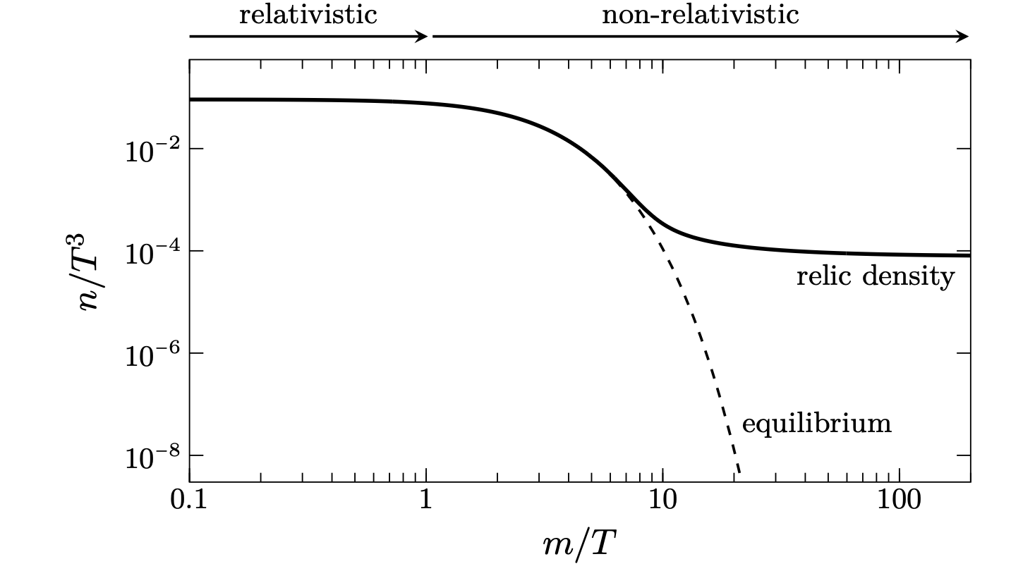
As we discussed earlier, in equilibrium, the number density of non-relativistic particles scales as \[ n \propto T^{3/2} e^{ -m/T } \] or is exponentially suppressed. This suppression can be simply thought of as annihilation removing particles and not enough energy in the thermal bath to produce new particles. However, this behavior is complicated by the expansion rate of the Universe. If the rate of the interactions keeping the particle in thermal equilibrium \(\Gamma\) becomes comparable to the Hubble expansion, then the annihilations get suppressed and the number density can freeze out (factoring out the cosmic expansion).
We can therefore summarize two regimes here:
- \(\Gamma \gg H\) : equilibrium
- \(\Gamma \ll H\) : Frozen out
The figure below captures this schematically.
This freezing out mechanism is responsible for a number of effects in cosmology
- Estimating the residual dark matter density for WIMPs and other thermally produced particles.
- Recombination
- The neutron density in BBN
- Baryogenesis
23.1 The Boltzmann Equation
These effects are captured by the Boltzmann equation \[ \frac{1}{a^{3}} \frac{d(n a^{3})}{dt} = C \] The LHS just captures the dilution of the density of particles as the Universe expands, while the right hand side captures the effect of interactions.
To be more specific, let us consider two-body interactions \[ 1 + 2 \leftrightarrow 3 + 4 \] and suppose we are interested in tracking particle 1. We then have \[ \frac{1}{a^{3}} \frac{d(n a^{3})}{dt} = -\alpha n_{1} n_{2} + \beta n_{3} n_{4} \] Using detailed balance, we estimate \[ \beta = \left( \frac{n_{1} n_{2}}{n_{3} n_{4}} \right)_\text{eq} \alpha \] which gives \[ \frac{1}{a^{3}} \frac{d(n a^{3})}{dt} = -\langle \sigma v\rangle \left[ n_{1} n_{2} - \left( \frac{n_{1} n_{2}}{n_{3} n_{4}} \right)_\text{eq} n_{3} n_{4} \right] \] where we have introduced the thermally averaged cross-section for \(\alpha\). While this is in terms of a physical density, it is convenient to write this in terms of the comoving density \(N_{i} \equiv n_{i}/{s}\), where we use the entropy density to track the expansion. This yields (using the definition of the Hubble parameter) \[ \frac{d \ln N_{1}}{d \ln a} = - \frac{\Gamma_{1}}{H} \left[ 1 - \left( \frac{N_{1} N_{2}}{N_{3} N_{4}} \right)_\text{eq} \frac{N_{3} N_{4}}{N_{1} N_{2}} \right] \] where \[ \Gamma = \langle \sigma v\rangle n_{2} \]
This captures our intuition - when \(\Gamma \gg H\) , the system is in equilibrium, while in the opposite limit, \(N_{1} \to \text{constant}\).
23.2 Thermal Relic Density of Dark Matter
Suppose we had a dark matter candidate \(X\) with the following reaction \[ X + \bar{X} \leftrightarrow l + \bar{l} \] where \(l\) is just a light SM particle. We will assume that \(l\) is tightly coupled to the thermal bath, so the number density is in equilibrium. We also assume no asymmetry between \(X\) and \(\bar{X}\), so that their number densities are equal. Finally, we assume that there are no additional annihilations taking place, so that \(T \propto a^{-1}\) (see our previous discussion).
The Boltzmann equation is then \[ \frac{1}{a^{3}} \frac{d(n a^{3})}{dt} = -\langle \sigma v\rangle \left[ n_{X}^{2} - (n_{X})_\text{eq}^{2} \right] \] Now for some convenient definitions
- \(Y \equiv n_{X}/T^3\) : this tracks the comoving number density
- A new time variable \(x \equiv M_{x}/T\), where \(dx/dt = H x\).
Finally, the Friedmann equation can be written as \[
H = \frac{H(M_{X})}{x^2}
\] Putting all this together and defining \[
\lambda \equiv \frac{\Gamma(M_{X})}{H(M_{X})} = \frac{M_{X}^{3} \langle \sigma v\rangle}{H(M_{X})}
\] we get \[
\frac{dY}{dx} = -\frac{\lambda}{x^2} \left[ Y^{2} - Y_\text{eq}^{2} \right]
\] The numerical solution for this gives 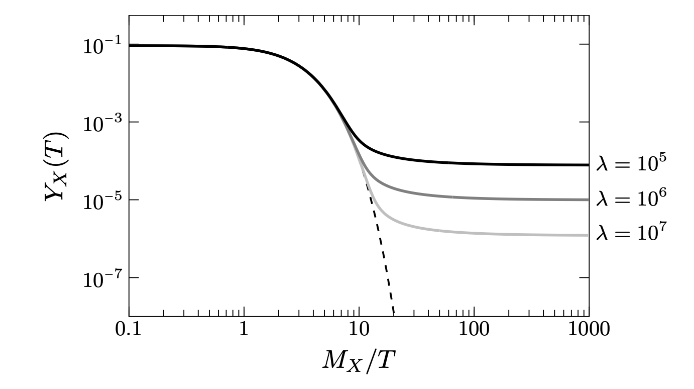
With a little more effort, we then get \[ \Omega_{X} \sim 0.1 \frac{x_{f}}{\sqrt{ g_{*}(M_{X}) }} \frac{10^{-8} \text{GeV}^{-2}}{\langle \sigma v\rangle} \] where \(x_{f} \sim 10\) is the rough freeze out time. If we choose \[ \sqrt{ \langle \sigma v\rangle } \sim 10^{-4} \text{GeV}^{-1} \sim 0.1 \sqrt{ G_{F} } \] we get a dark matter density similar to what we observe.