Code
import numpy as np
import matplotlib.pyplot as plt
import matplotlib.patches as patches
from matplotlib.colors import NormalizeIn the previous lecture, we started from the collisionless Boltzmann (Vlasov) equation coupled to the Poisson equation — the Vlasov–Poisson system — which governs the evolution of collisionless dark matter in comoving coordinates \(\mathbf{x}\) (with \(\mathbf{r} = a(t)\mathbf{x}\)). Since the 6D phase space is too large to simulate directly, we Monte-Carlo sample the distribution function with \(N\) particles in a periodic box of comoving side \(L\), each carrying a mass \[ m_p = \Omega_m \bar{\rho} \frac{L^3}{N} \]
We then derived the equations of motion for each particle. Starting from the full Lagrangian \(L = \frac{1}{2}m|\dot{a}\mathbf{x} + a\dot{\mathbf{x}}|^2 - m\varphi\), we decomposed the gravitational potential as \(\varphi = \varphi_{\text{bg}} + \Phi\) where \(\varphi_{\text{bg}} = \frac{2\pi}{3}G\bar{\rho}a^2|\mathbf{x}|^2\). The background and cross terms cancel exactly (using the Friedmann equation \(\ddot{a}/a = -4\pi G \bar{\rho}/3\)), leaving the peculiar Lagrangian: \[ \mathcal{L}_{\text{pec}} = \frac{1}{2} m a^2 \dot{\mathbf{x}}^2 - m \Phi(\mathbf{x}, t) \] where \(\Phi\) is the peculiar potential satisfying the Poisson equation: \[ \nabla^2 \Phi = 4\pi G \bar{\rho} a^2 \delta \]
The conjugate momentum is \(\mathbf{p} = ma^2\dot{\mathbf{x}}\), and the Euler–Lagrange equation gives \[ \ddot{\mathbf{x}} + 2\frac{\dot{a}}{a}\dot{\mathbf{x}} = -\frac{1}{a^2}\nabla_x \Phi \] with the familiar Hubble drag term \(2H\dot{\mathbf{x}}\).
We also saw the total derivative trick: adding \(d/dt(\frac{1}{2}ma\dot{a}|\mathbf{x}|^2)\) to \(\mathcal{L}_{\text{pec}}\) gives \(\mathcal{L}'\) with conjugate momentum \(\mathbf{p}' = ma\dot{\mathbf{r}}\) (proportional to the total velocity), and the simpler equations \(d\mathbf{x}/dt = \mathbf{p}'/(ma^2)\), \(d\mathbf{p}'/dt = -m\nabla_x\Phi\) — no Hubble drag, but the momentum now includes the Hubble flow.
The task is now to integrate these equations efficiently and stably over cosmological timescales — which brings us to symplectic methods.
The equations of motion derived from \(\mathcal{L}_{\text{pec}}\) are Hamiltonian, and Hamiltonian systems have a fundamental geometric property: they preserve the symplectic form on phase space. Loosely speaking, this means that the flow of trajectories preserves phase-space volume (Liouville’s theorem) and the area of any canonical \((x_i, p_i)\) pair.
A generic ODE integrator (e.g., Runge–Kutta) does not respect this structure. Over many timesteps, such integrators introduce systematic drift in conserved quantities — the energy “random walks” away from its true value. For cosmological simulations, where we may take \(10^3\)–\(10^4\) timesteps, this secular drift is unacceptable.
Symplectic integrators are constructed to exactly preserve the symplectic structure at each step. The key consequence: while the energy at each step has an \(\mathcal{O}(\Delta t^n)\) error (where \(n\) is the order of the integrator), this error is bounded — it oscillates rather than drifts. There is no secular growth.
In cosmology, the Hamiltonian is explicitly time-dependent (through \(a(t)\)), so there is no conserved energy. Symplecticity is still valuable, however: it preserves phase-space structure, prevents artificial dissipation or heating of particle orbits, and maintains the correct topology of trajectories. The composition of symplectomorphisms is itself a symplectomorphism — this is the mathematical property that makes the whole approach work.
For testing purposes, there exists a Layzer–Irvine equation that predicts \(dE/dt\) given the expansion history — one can integrate this alongside the simulation as a consistency check. We will not derive it here.
Consider a Hamiltonian of the form \[ H = A(\mathbf{p}) + B(\mathbf{x}) \] Each piece alone generates a trivially solvable flow:
The idea of symplectic splitting is to approximate the full evolution by alternating these sub-steps. Each sub-step is an exact symplectomorphism (it solves a Hamiltonian system exactly), and the composition of symplectomorphisms is a symplectomorphism. So the overall integrator is automatically symplectic, regardless of the step size.
The splitting approximation can be understood through the BCH formula. For operators \(\hat{A}\) and \(\hat{B}\), \[ e^{\hat{A}\Delta t} \, e^{\hat{B}\Delta t} = e^{(\hat{A}+\hat{B})\Delta t + \frac{1}{2}[\hat{A},\hat{B}]\Delta t^2 + \cdots} \] The leading error is \(\mathcal{O}(\Delta t^2)\), giving a first-order integrator. By symmetrizing — taking a half-step, a full step, and another half-step — the odd-order error terms cancel, yielding second-order accuracy.
The most common choice for cosmological simulations is the Kick-Drift-Kick (KDK) leapfrog:
This is a second-order symplectic integrator: the position and force errors are \(\mathcal{O}(\Delta t^2)\) per step.
The alternative Drift-Kick-Drift (DKD) ordering is equally valid and has the same formal accuracy. KDK is preferred in practice because after each full step, the positions and momenta are synchronized at the same time — making it easy to output snapshots and diagnostics. In DKD, positions lead momenta by a half step, requiring an extra synchronization step for output.
The peculiar Lagrangian uses coordinate time \(t\), which leads to explicit time-dependence through \(a(t)\) and introduces Hubble drag terms in the equation of motion. We can eliminate this by choosing a better time variable.
Define \[ \eta \equiv \ln a \] so that \(d\eta = da/a = (da/dt)/a \, dt = H \, dt\), or equivalently, \(dt = d\eta / H\). This is a monotonic reparametrization of time (as long as \(H > 0\), i.e., the universe is expanding).
We now re-derive the Lagrangian, conjugate momentum, and Hamiltonian in this new time variable.
The action is invariant under reparametrization of time. Starting from \[ S = \int \left[ \frac{1}{2} m a^2 \dot{\mathbf{x}}^2 - m\Phi \right] dt \] we substitute \(dt = d\eta/H\) and \(\dot{\mathbf{x}} = (d\mathbf{x}/d\eta)(d\eta/dt) = H \mathbf{x}'\) where primes denote \(d/d\eta\): \[ S = \int \left[ \frac{1}{2} m a^2 H^2 \mathbf{x}'^2 - m\Phi \right] \frac{d\eta}{H} = \int \left[ \frac{1}{2} m a^2 H \, \mathbf{x}'^2 - \frac{m\Phi}{H} \right] d\eta \]
Reading off the \(\eta\)-Lagrangian: \[ \tilde{\mathcal{L}} = \frac{1}{2} m a^2 H \, \mathbf{x}'^2 - \frac{m\Phi}{H} \]
The conjugate momentum with respect to \(\eta\) is \[ \mathbf{p} = \frac{\partial \tilde{\mathcal{L}}}{\partial \mathbf{x}'} = m a^2 H \, \mathbf{x}' \] Since \(\mathbf{x}' = d\mathbf{x}/d\eta = \dot{\mathbf{x}}/H\), this gives \[ \mathbf{p} = m a^2 \dot{\mathbf{x}} \] This is the same conjugate momentum as in the original (\(t\)-time) Lagrangian — it is proportional to the peculiar velocity \(\mathbf{v}_{\text{pec}} = a \dot{\mathbf{x}}\): \[ \mathbf{p} = m a \, \mathbf{v}_{\text{pec}} \]
This momentum is convenient for computing redshift-space positions. If \(\hat{\mathbf{n}}\) is the line-of-sight direction, the redshift-space coordinate is \[ \mathbf{s} = \mathbf{x} + \hat{\mathbf{n}} \frac{p_\parallel}{m a^2 H} = \mathbf{x} + \hat{\mathbf{n}} \frac{v_{\text{pec},\parallel}}{a H} \] Having \(\mathbf{p} = m a^2 \dot{\mathbf{x}}\) directly available from the integrator makes this trivial to evaluate.
To construct the Hamiltonian, we perform the Legendre transform: \[ \tilde{H} = \mathbf{p} \cdot \mathbf{x}' - \tilde{\mathcal{L}} \] First, express \(\mathbf{x}'\) in terms of \(\mathbf{p}\): \[ \mathbf{x}' = \frac{\mathbf{p}}{m a^2 H} \] Then: \[ \mathbf{p} \cdot \mathbf{x}' = \frac{\mathbf{p}^2}{m a^2 H} \] \[ \tilde{\mathcal{L}} = \frac{1}{2} \frac{\mathbf{p}^2}{m a^2 H} - \frac{m\Phi}{H} \] Therefore: \[ \tilde{H} = \frac{\mathbf{p}^2}{m a^2 H} - \frac{1}{2}\frac{\mathbf{p}^2}{m a^2 H} + \frac{m\Phi}{H} \] \[ \boxed{\tilde{H} = \underbrace{\frac{\mathbf{p}^2}{2 m a^2 H}}_{\displaystyle A(\mathbf{p}, \eta)} + \underbrace{\frac{m\Phi(\mathbf{x})}{H}}_{\displaystyle B(\mathbf{x}, \eta)}} \]
This is the key result: the Hamiltonian is separable into a kinetic term \(A\) depending only on \(\mathbf{p}\) (and \(\eta\)) and a potential term \(B\) depending only on \(\mathbf{x}\) (and \(\eta\)). This separability is exactly what we need for the symplectic splitting to work.
The explicit time-dependence through \(H(\eta)\) and \(a(\eta)\) does not spoil the splitting — what matters is that for a fixed value of \(\eta\), the Hamiltonian separates into a function of \(\mathbf{p}\) alone plus a function of \(\mathbf{x}\) alone. The time-dependence of the coefficients simply means that the drift and kick factors vary from step to step.
From \(\tilde{H}\), Hamilton’s equations in the \(\eta\) variable are: \[ \frac{d\mathbf{x}}{d\eta} = \frac{\partial \tilde{H}}{\partial \mathbf{p}} = \frac{\mathbf{p}}{m a^2 H} \] \[ \frac{d\mathbf{p}}{d\eta} = -\frac{\partial \tilde{H}}{\partial \mathbf{x}} = -\frac{m \nabla\Phi}{H} \]
These equations have no Hubble drag term — the friction that appeared in the coordinate-time formulation has been absorbed into the choice of time variable and conjugate momentum.
In the KDK scheme, the drift and kick sub-steps require integrating Hamilton’s equations with either \(B = 0\) (drift) or \(A = 0\) (kick) over an interval in \(\eta\). Since \(A\) and \(B\) have explicit \(\eta\)-dependence through \(a\) and \(H\), these sub-steps involve integrals.
Drift step (from \(a_1\) to \(a_2\), with \(\mathbf{p}\) fixed): \[ \Delta \mathbf{x} = \frac{\mathbf{p}}{m} \int_{a_1}^{a_2} \frac{d\eta}{a^2 H} = \frac{\mathbf{p}}{m} \int_{a_1}^{a_2} \frac{da}{a^3 H(a)} \] where we used \(d\eta = da/a\). We define the drift factor: \[ \boxed{D(a_1, a_2) \equiv \int_{a_1}^{a_2} \frac{da}{a^3 H(a)}} \]
Kick step (from \(a_1\) to \(a_2\), with \(\mathbf{x}\) fixed): \[ \Delta \mathbf{p} = -m \nabla\Phi \int_{a_1}^{a_2} \frac{d\eta}{H} = -m \nabla\Phi \int_{a_1}^{a_2} \frac{da}{a H(a)} \] We define the kick factor: \[ \boxed{K(a_1, a_2) \equiv \int_{a_1}^{a_2} \frac{da}{a H(a)}} \]
We converted from \(d\eta\) to \(da/a\) for practical reasons: the Hubble parameter \(H(a)\) is a known function of \(a\) (from the Friedmann equation), making the integrands explicit. In the \(\eta\) variable, one would need \(H\) as a function of \(\eta = \ln a\), which is the same information in a slightly less convenient form.
For an Einstein–de Sitter (EdS) universe (\(\Omega_m = 1\), \(\Omega_\Lambda = 0\)), the Friedmann equation gives \[ H(a) = H_0 \, a^{-3/2} \]
The drift and kick factors then have closed-form expressions.
Drift factor: \[ D(a_1, a_2) = \int_{a_1}^{a_2} \frac{da}{a^3 \cdot H_0 a^{-3/2}} = \frac{1}{H_0} \int_{a_1}^{a_2} \frac{da}{a^{3/2}} = \frac{1}{H_0} \left[ -\frac{2}{\sqrt{a}} \right]_{a_1}^{a_2} \] \[ D_{\text{EdS}}(a_1, a_2) = \frac{2}{H_0} \left( \frac{1}{\sqrt{a_1}} - \frac{1}{\sqrt{a_2}} \right) \]
Kick factor: \[ K(a_1, a_2) = \int_{a_1}^{a_2} \frac{da}{a \cdot H_0 a^{-3/2}} = \frac{1}{H_0} \int_{a_1}^{a_2} a^{1/2} \, da = \frac{1}{H_0} \left[ \frac{2}{3} a^{3/2} \right]_{a_1}^{a_2} \] \[ K_{\text{EdS}}(a_1, a_2) = \frac{2}{3 H_0} \left( a_2^{3/2} - a_1^{3/2} \right) \]
For a general flat \(\Lambda\)CDM cosmology: \[ H(a) = H_0 \sqrt{\Omega_m \, a^{-3} + \Omega_\Lambda} \]
The drift and kick integrals become: \[ D(a_1, a_2) = \int_{a_1}^{a_2} \frac{da}{a^3 H_0 \sqrt{\Omega_m a^{-3} + \Omega_\Lambda}} \] \[ K(a_1, a_2) = \int_{a_1}^{a_2} \frac{da}{a H_0 \sqrt{\Omega_m a^{-3} + \Omega_\Lambda}} \]
These generally do not have closed-form solutions and must be evaluated numerically.
In practice, production \(N\)-body codes precompute \(D(a)\) and \(K(a)\) as lookup tables at startup (evaluated from some initial \(a_i\) to a grid of \(a\) values using numerical quadrature). During the simulation, the drift and kick factors for any interval \([a_1, a_2]\) are obtained by table lookup and subtraction: \(D(a_1, a_2) = D(a_2) - D(a_1)\).
The three natural Lagrangian formulations for cosmological \(N\)-body simulations differ in their choice of time variable and conjugate momentum:
| \(\mathcal{L}_{\text{pec}}\) | \(\mathcal{L}'\) (total deriv.) | \(\tilde{\mathcal{L}}\) (\(\ln a\) time) | |
|---|---|---|---|
| Time variable | \(t\) | \(t\) | \(\eta = \ln a\) |
| Conjugate momentum | \(ma^2\dot{\mathbf{x}}\) | \(ma\dot{\mathbf{r}}\) | \(ma^2\dot{\mathbf{x}}\) |
| Physical meaning of \(p\) | \(\propto \mathbf{v}_{\text{pec}}\) | \(\propto\) total velocity | \(\propto \mathbf{v}_{\text{pec}}\) |
| Hubble drag in EOM | Yes | No | No |
| RSD convenience | Direct | Requires subtracting \(H\mathbf{x}\) | Direct |
| Hamiltonian separable? | Yes | Yes | Yes |
| Common use | Textbook derivations | Analytical work | Simulation codes |
The \(\tilde{\mathcal{L}}\) formulation with \(\eta = \ln a\) is preferred for simulations: the absence of Hubble drag simplifies the integrator, the conjugate momentum directly gives the peculiar velocity, and \(\eta\) provides a natural logarithmic time-stepping (equal steps in \(\eta\) correspond to equal expansion factors, giving finer resolution at early times when structures are forming rapidly).
Bringing it all together, a single KDK leapfrog step advancing from \(a_n\) to \(a_{n+1}\) (with midpoint \(a_{n+1/2}\)) proceeds as:
Step 1 — Half Kick: \[ \mathbf{p}_{n+1/2} = \mathbf{p}_n - m \nabla\Phi(\mathbf{x}_n) \, K(a_n, a_{n+1/2}) \]
Step 2 — Full Drift: \[ \mathbf{x}_{n+1} = \mathbf{x}_{n} + \frac{\mathbf{p}_{n+1/2}}{m} \, D(a_n, a_{n+1}) \]
Step 3 — Half Kick:
Compute \(\nabla\Phi(\mathbf{x}_{n+1})\) from the particle positions at \(\mathbf{x}_{n+1}\) (this is where the Poisson solver enters — to be discussed in later sections), then: \[ \mathbf{p}_{n+1} = \mathbf{p}_{n+1/2} - m \nabla\Phi(\mathbf{x}_{n+1}) \, K(a_{n+1/2}, a_{n+1}) \]
The force evaluation (computing \(\nabla\Phi\) from the particle distribution) is by far the most expensive part of each timestep. The KDK ordering means we need exactly one force evaluation per step — the force at the end of one step provides the first half-kick of the next step. This is a crucial practical advantage. How we compute this force efficiently using the Particle-Mesh method (CIC interpolation + FFT-based Poisson solver) is the subject of the next sections.
Before diving into the Particle-Mesh algorithm, let us set up our computational environment. We will use JAX for the simulation code (to be developed in later sections), but for now we only need NumPy and Matplotlib.
import numpy as np
import matplotlib.pyplot as plt
import matplotlib.patches as patches
from matplotlib.colors import NormalizeThe KDK integrator needs the gravitational force \(\nabla\Phi\) at every particle position, which requires solving the Poisson equation \[ \nabla^2 \Phi = 4\pi G \bar{\rho} a^2 \delta \] The Particle-Mesh (PM) method solves this on a regular grid using FFTs, which gives \(\mathcal{O}(N_g \log N_g)\) scaling (where \(N_g\) is the number of grid cells) rather than the \(\mathcal{O}(N^2)\) cost of direct particle-particle summation.
The PM pipeline has three steps:
Steps 1 and 3 require a scheme for transferring quantities between particles (at arbitrary positions) and grid points (at fixed locations). The choice of scheme controls the accuracy, smoothness, and isotropy of the forces.
The simplest approach: assign each particle’s entire mass to the single nearest grid point.
For a 1D grid with spacing \(h\) and grid points at \(x_j = jh\), a particle at position \(x_p\) contributes to the grid as: \[ \rho_j \mathrel{+}= m_p \cdot \begin{cases} 1 & \text{if } |x_p - x_j| < h/2 \\ 0 & \text{otherwise} \end{cases} \]
This is just a zeroth-order (piecewise constant) interpolation. It is fast but produces a very noisy density field — the density jumps discontinuously every time a particle crosses a cell boundary, and these discontinuities propagate into discontinuous forces.
Cloud-in-Cell is a first-order (piecewise linear) scheme that spreads each particle’s mass across the \(2^d\) nearest grid points (where \(d\) is the number of dimensions), weighted by the overlap volume.
In 1D, a particle at \(x_p\) contributes to the two bracketing grid points \(x_j\) and \(x_{j+1}\) with weights: \[ W(x_p, x_j) = \begin{cases} 1 - |x_p - x_j|/h & \text{if } |x_p - x_j| < h \\ 0 & \text{otherwise} \end{cases} \]
The weight is just a triangle (tent) function — linearly interpolating between the two nearest grid points. In \(d\) dimensions, the weight factorizes: \[ W(\mathbf{x}_p, \mathbf{x}_j) = \prod_{i=1}^{d} W(x_{p,i}, x_{j,i}) \] so in 3D each particle contributes to \(2^3 = 8\) grid points.
A crucial requirement: the same scheme must be used for mass assignment (particles → grid) and force interpolation (grid → particles). Using different schemes breaks Newton’s third law — a particle would not feel the same force it exerts — leading to self-forces and momentum non-conservation. This is sometimes called the “transpose” requirement: the interpolation operator must be the transpose of the assignment operator.
To build intuition, let us visualize how CIC works. We place a few particles on a 1D grid and show how each particle’s mass is split between neighboring grid points.
fig, axes = plt.subplots(2, 1, figsize=(10, 6), sharex=True,
                         gridspec_kw={'height_ratios': [2, 1]})

# Grid setup
ngrid = 8
h = 1.0  # cell spacing
grid_x = np.arange(ngrid) * h + h/2  # cell centers

# A few example particles at arbitrary positions
particles = np.array([1.2, 2.8, 3.1, 5.7])
colors_p = plt.cm.Set1(np.linspace(0, 0.4, len(particles)))

# --- Top panel: individual particle contributions ---
ax = axes[0]

# Draw grid lines
for gx in grid_x:
    ax.axvline(gx, color='0.85', lw=0.5, zorder=0)

# Cell boundaries
for i in range(ngrid + 1):
    ax.axvline(i * h, color='0.7', lw=0.5, ls='--', zorder=0)

# For each particle, show the CIC weights
bar_width = 0.15
total_density = np.zeros(ngrid)

for ip, xp in enumerate(particles):
    weights = np.zeros(ngrid)
    for j in range(ngrid):
        dx = abs(xp - grid_x[j]) / h
        if dx < 1.0:
            weights[j] = 1.0 - dx
    total_density += weights

    offset = (ip - len(particles)/2 + 0.5) * bar_width
    ax.bar(grid_x + offset, weights, width=bar_width, alpha=0.7,
           color=colors_p[ip], label=f'$x_p = {xp}$', zorder=2)

    # Draw the particle position
    ax.plot(xp, -0.06, marker='^', ms=10, color=colors_p[ip],
            clip_on=False, zorder=5)

# Draw grid points
ax.plot(grid_x, np.zeros(ngrid), 'ko', ms=6, zorder=3)

ax.set_ylabel('CIC weight $W(x_p, x_j)$')
ax.set_ylim(-0.02, 1.05)
ax.legend(loc='upper right', fontsize=9, ncol=2)
ax.set_title('Individual particle contributions')

# --- Bottom panel: total deposited density ---
ax = axes[1]

for gx in grid_x:
    ax.axvline(gx, color='0.85', lw=0.5, zorder=0)
for i in range(ngrid + 1):
    ax.axvline(i * h, color='0.7', lw=0.5, ls='--', zorder=0)

ax.bar(grid_x, total_density, width=0.6, color='0.4', alpha=0.7, zorder=2)
ax.plot(grid_x, np.zeros(ngrid), 'ko', ms=6, zorder=3)

# Show particles
for ip, xp in enumerate(particles):
    ax.plot(xp, -0.08, marker='^', ms=10, color=colors_p[ip],
            clip_on=False, zorder=5)

ax.set_xlabel('$x$')
ax.set_ylabel('Total density')
ax.set_title('Sum over all particles')

plt.tight_layout()
plt.show()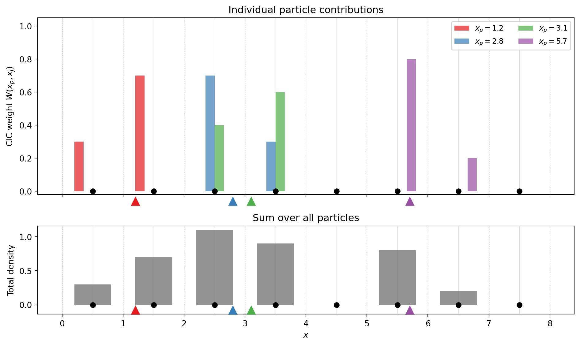
In 2D, each particle deposits mass onto the four corners of its enclosing cell. The weight at each corner is the product of the 1D weights in each direction — geometrically, this is the area of the rectangle diagonally opposite to that corner.
fig, ax = plt.subplots(1, 1, figsize=(6, 6))

# Grid
ngrid = 5
h = 1.0
for i in range(ngrid + 1):
    ax.axhline(i * h, color='0.8', lw=0.5)
    ax.axvline(i * h, color='0.8', lw=0.5)

# Grid points (cell centers)
for i in range(ngrid):
    for j in range(ngrid):
        ax.plot(i * h + h/2, j * h + h/2, 'ko', ms=5, zorder=3)

# Particle position
xp, yp = 2.3, 2.7

# Enclosing cell corners (grid point indices)
# Grid points at cell centers: x_j = j*h + h/2
# Find the two nearest in each direction
jx = int((xp - h/2) / h)  # left grid point index
jy = int((yp - h/2) / h)  # lower grid point index

corners = [(jx, jy), (jx+1, jy), (jx, jy+1), (jx+1, jy+1)]
corner_coords = [(c[0]*h + h/2, c[1]*h + h/2) for c in corners]

# CIC weights
dx = (xp - corner_coords[0][0]) / h
dy = (yp - corner_coords[0][1]) / h

weights = [
    (1 - dx) * (1 - dy),  # lower-left
    dx * (1 - dy),         # lower-right
    (1 - dx) * dy,         # upper-left
    dx * dy,               # upper-right
]

# Color patches showing the "opposite area" interpretation
# For each corner, the weight = area of rectangle on the opposite side
patch_specs = [
    # (lower-left corner, opposite area is upper-right)
    (xp, yp, corner_coords[3][0] - xp + h/2, corner_coords[3][1] - yp + h/2),
    # (lower-right corner, opposite area is upper-left)
    (corner_coords[0][0] - h/2, yp, xp - corner_coords[0][0] + h/2, corner_coords[3][1] - yp + h/2),
    # (upper-left corner, opposite area is lower-right)
    (xp, corner_coords[0][1] - h/2, corner_coords[3][0] - xp + h/2, yp - corner_coords[0][1] + h/2),
    # (upper-right corner, opposite area is lower-left)
    (corner_coords[0][0] - h/2, corner_coords[0][1] - h/2, xp - corner_coords[0][0] + h/2, yp - corner_coords[0][1] + h/2),
]

cmap = plt.cm.Blues
norm = Normalize(vmin=0, vmax=max(weights) * 1.5)
labels_pos = ['lower-left', 'lower-right', 'upper-left', 'upper-right']

for i, ((cx, cy), w, ps) in enumerate(zip(corner_coords, weights, patch_specs)):
    # Shaded rectangle (opposite area)
    rect = patches.Rectangle((ps[0], ps[1]), ps[2], ps[3],
                              facecolor=cmap(norm(w)), edgecolor='steelblue',
                              lw=1.5, alpha=0.5, zorder=1)
    ax.add_patch(rect)

    # Weight label at grid point
    ax.annotate(f'$W = {w:.2f}$', (cx, cy),
                textcoords='offset points', xytext=(12, 8),
                fontsize=11, fontweight='bold', color='steelblue',
                bbox=dict(boxstyle='round,pad=0.2', fc='white', ec='steelblue', alpha=0.8))

    # Highlight grid point
    ax.plot(cx, cy, 'o', ms=10, color='steelblue', zorder=4)

# Particle
ax.plot(xp, yp, 'r*', ms=18, zorder=5)
ax.annotate(f'particle\n$({xp}, {yp})$', (xp, yp),
            textcoords='offset points', xytext=(-50, -30),
            fontsize=10, color='red',
            arrowprops=dict(arrowstyle='->', color='red'))

# Dashed lines from particle to cell edges
ax.axhline(yp, color='red', ls=':', lw=0.8, alpha=0.5)
ax.axvline(xp, color='red', ls=':', lw=0.8, alpha=0.5)

# Dimension annotations
y_bottom = corner_coords[0][1]
ax.annotate('', xy=(xp, y_bottom - 0.35), xytext=(corner_coords[0][0], y_bottom - 0.35),
            arrowprops=dict(arrowstyle='<->', color='0.3', lw=1.5))
ax.text((xp + corner_coords[0][0])/2, y_bottom - 0.45, f'$dx={dx:.1f}$',
        ha='center', fontsize=10, color='0.3')

ax.annotate('', xy=(corner_coords[1][0], y_bottom - 0.35), xytext=(xp, y_bottom - 0.35),
            arrowprops=dict(arrowstyle='<->', color='0.3', lw=1.5))
ax.text((xp + corner_coords[1][0])/2, y_bottom - 0.45, f'$1-dx={1-dx:.1f}$',
        ha='center', fontsize=10, color='0.3')

ax.set_xlim(0.5, 4.5)
ax.set_ylim(1.0, 5.0)
ax.set_aspect('equal')
ax.set_xlabel('$x$')
ax.set_ylabel('$y$')

plt.tight_layout()
plt.show()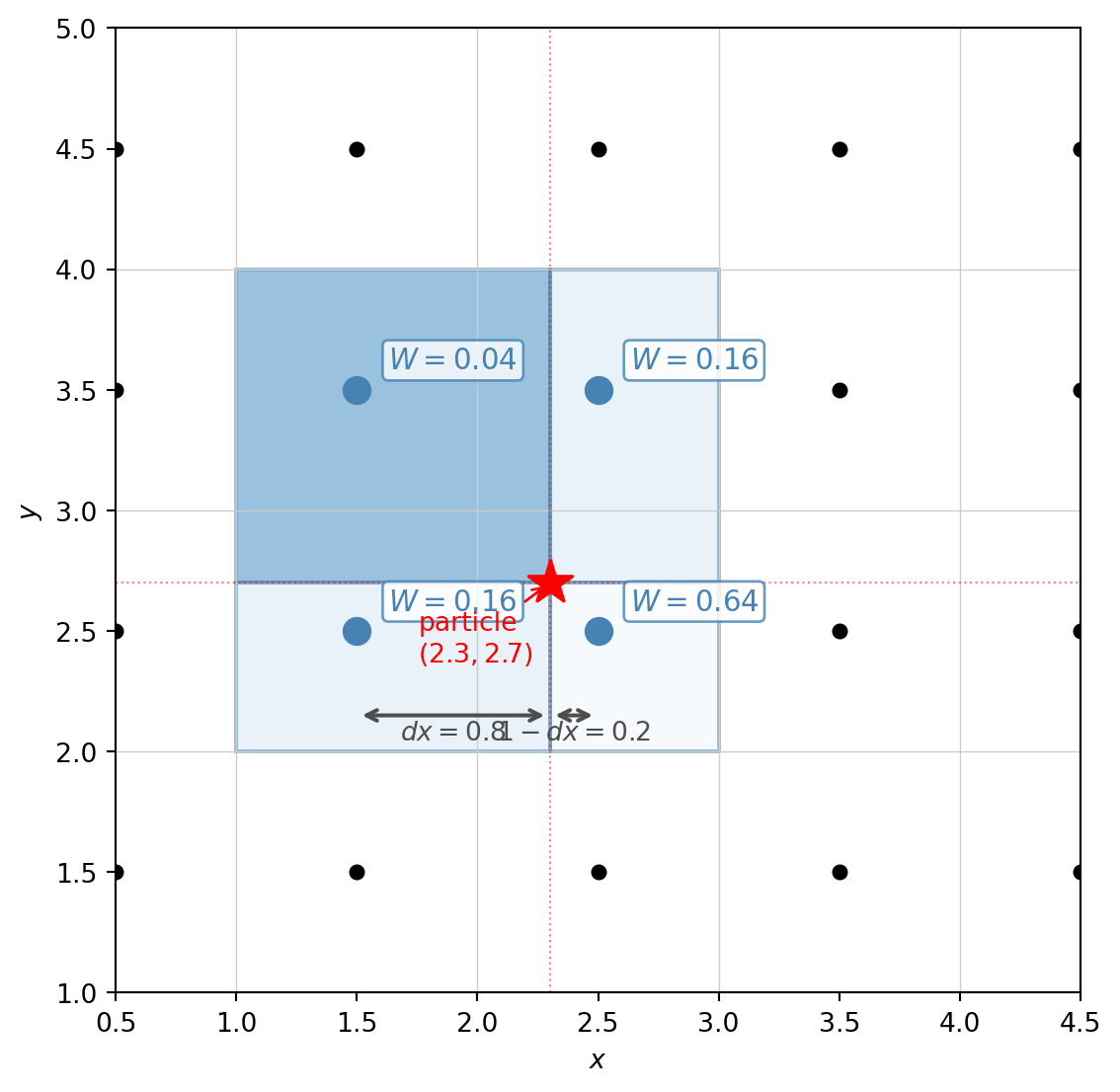
CIC is the standard choice for PM codes because it strikes a good balance:
| Scheme | Order | Grid points per particle | Density continuity | Force continuity |
|---|---|---|---|---|
| NGP | 0 | \(1\) | Discontinuous | Discontinuous |
| CIC | 1 | \(2^d\) | Continuous (\(C^0\)) | Discontinuous |
| TSC | 2 | \(3^d\) | \(C^1\) | Continuous |
Higher-order schemes (TSC = Triangular Shaped Cloud, and beyond) give smoother forces but spread each particle over more grid points, increasing the cost of the assignment and interpolation steps. CIC is almost universally used in production PM and TreePM codes — the force discontinuity is at the grid scale and is subdominant to the grid-scale force resolution limit inherent in the PM method anyway.
There is a clean mathematical way to think about the full NGP → CIC → TSC hierarchy. NGP assigns mass using a top-hat window of width \(h\) (the “zeroth-order B-spline”). CIC convolves this top-hat with itself, producing the triangle/tent function — the first-order B-spline. TSC convolves once more, producing the second-order B-spline (a piecewise quadratic). Each successive convolution gains one order of smoothness. In Fourier space, convolution becomes multiplication, so the CIC window function is \(\tilde{W}(k) = \mathrm{sinc}^2(kh/2)\), compared to \(\mathrm{sinc}(kh/2)\) for NGP — the CIC window suppresses small-scale power more aggressively, which is the price of smoother forces.
Once we have solved for \(\Phi\) on the grid (next section), we need the force \(\mathbf{F} = -m\nabla\Phi\) at each particle position. As emphasized above, we must use the same CIC weights to interpolate the force back to the particles: \[ \mathbf{F}(\mathbf{x}_p) = -m \sum_j W(\mathbf{x}_p, \mathbf{x}_j) \, \nabla\Phi(\mathbf{x}_j) \] where the sum runs over the \(2^d\) grid points surrounding particle \(p\), and the gradient \(\nabla\Phi\) on the grid is computed by finite differences (or, equivalently, by multiplying by \(i\mathbf{k}\) in Fourier space before transforming back — more on this in the next section).
This completes the assignment/interpolation infrastructure. We now turn to the middle step of the PM pipeline: solving the Poisson equation on the grid using FFTs.
We need to solve \[ \nabla^2 \Phi = 4\pi G \bar{\rho} a^2 \delta \] on a periodic grid. Periodicity is the key simplification: the eigenfunctions of \(\nabla^2\) on a periodic domain are plane waves \(e^{i\mathbf{k}\cdot\mathbf{x}}\), so the Poisson equation becomes algebraic in Fourier space.
Before proceeding, we need to be precise about our Fourier transform conventions. On a grid of \(N_g\) points in each dimension with spacing \(h = L/N_g\), the discrete Fourier transform (DFT) and its inverse are:
\[ \hat{f}_\mathbf{k} = \sum_{\mathbf{n}} f_\mathbf{n} \, e^{-2\pi i \, \mathbf{k}\cdot\mathbf{n}/N_g} \] \[ f_\mathbf{n} = \frac{1}{N_g^d} \sum_{\mathbf{k}} \hat{f}_\mathbf{k} \, e^{+2\pi i \, \mathbf{k}\cdot\mathbf{n}/N_g} \]
where \(\mathbf{n}\) indexes grid points and \(\mathbf{k}\) indexes wavenumber bins. This is the convention used by NumPy’s np.fft.fftn and np.fft.ifftn (and JAX’s jnp.fft.fftn), with the \(1/N_g^d\) normalization on the inverse transform.
In physics we work with the continuous Fourier transform pair (in 1D for clarity): \[ \hat{f}(k) = \int_{-\infty}^{\infty} f(x) \, e^{-ikx} \, dx \qquad f(x) = \int_{-\infty}^{\infty} \hat{f}(k) \, \frac{dk}{2\pi} \, e^{+ikx} \] On a periodic box of length \(L\) with \(N_g\) grid points at positions \(x_n = nh\) (where \(h = L/N_g\)), the integral becomes a Riemann sum: \[ \hat{f}(k) \approx \sum_{n=0}^{N_g-1} f(x_n) \, e^{-ik x_n} \, h \] The allowed wavenumbers are \(k = 2\pi m / L\) for integer \(m\). Substituting \(x_n = nh = nL/N_g\) and \(k = 2\pi m/L\): \[ \hat{f}(k_m) \approx h \sum_{n=0}^{N_g-1} f_n \, e^{-2\pi i \, mn/N_g} = h \, \hat{f}_m^{\text{DFT}} \] So the DFT output differs from the continuous transform by a factor of \(h\) (the grid spacing, which is the quadrature weight of the Riemann sum).
Similarly, for the inverse transform, the integral over \(dk/(2\pi)\) becomes a sum over discrete modes with spacing \(\Delta k = 2\pi/L\): \[ f(x_n) \approx \sum_{m} \hat{f}(k_m) \, e^{+ik_m x_n} \, \frac{\Delta k}{2\pi} = \frac{1}{L} \sum_m \hat{f}(k_m) \, e^{+2\pi i \, mn/N_g} \] Substituting \(\hat{f}(k_m) = h \, \hat{f}_m^{\text{DFT}}\): \[ f_n = \frac{h}{L} \sum_m \hat{f}_m^{\text{DFT}} \, e^{+2\pi i \, mn/N_g} = \frac{1}{N_g} \sum_m \hat{f}_m^{\text{DFT}} \, e^{+2\pi i \, mn/N_g} \] which is exactly the DFT inverse transform convention above.
In \(d\) dimensions, the volume element \(d^d x \to h^d\) gives:
\[ \boxed{\hat{f}(\mathbf{k}) = h^d \, \hat{f}_\mathbf{k}^{\text{DFT}}} \qquad \boxed{f(\mathbf{x}_\mathbf{n}) = h^{-d} \, f_\mathbf{n}^{\text{IDFT}}} \]
where \(h = L/N_g\) is the grid spacing. Here \(\hat{f}^{\text{DFT}}\) denotes the output of fftn, and \(f^{\text{IDFT}}\) denotes the output of ifftn when fed \(\hat{f}(\mathbf{k})\) (the continuous transform values). The forward relation says: multiply the fftn output by the volume element \(h^d\) to get the continuous transform. The inverse says: if you feed continuous Fourier coefficients into ifftn, multiply the result by \(h^{-d}\) to get the field values. The two factors are inverses of each other, as they must be.
If your equation is entirely in Fourier space (like the Poisson equation: divide \(\hat{\delta}\) by \(\hat{L}\) to get \(\hat{\Phi}\), then differentiate), the \(h^d\) factors cancel between the forward and inverse transforms and you can work directly with the DFT output — no extra factors needed.
The factors matter when you need to relate DFT output to a physical quantity with specific units. For example, the power spectrum: \[ P(k) = |\hat{\delta}(k)|^2 = h^{2d} \, |\hat{\delta}_\mathbf{k}^{\text{DFT}}|^2 \] or Parseval’s theorem relating a real-space integral to a Fourier-space sum. We will encounter this when setting up initial conditions from a power spectrum.
The DFT indices \(\mathbf{k}\) run over integers. The corresponding physical wavenumbers are \[
\mathbf{k}_{\text{phys}} = \frac{2\pi \mathbf{k}}{L}
\] The Nyquist frequency is \(k_{\text{Ny}} = \pi N_g / L = \pi / h\). Modes above this frequency are aliased. In NumPy, after np.fft.fftn, the wavenumber indices are ordered as \(k = 0, 1, \ldots, N_g/2, -N_g/2+1, \ldots, -1\); use np.fft.fftfreq(Ng, d=h) to get the physical frequencies directly.
Taking the DFT of the Poisson equation: \[ \widehat{\nabla^2 \Phi}_\mathbf{k} = (4\pi G \bar{\rho} a^2) \, \hat{\delta}_\mathbf{k} \]
The left-hand side requires the Fourier-space representation of \(\nabla^2\). On a continuous domain, \(\nabla^2 e^{i\mathbf{k}\cdot\mathbf{x}} = -k^2 e^{i\mathbf{k}\cdot\mathbf{x}}\), so one might use \(-k^2\). However, on a discrete grid we should use the Laplacian that is consistent with the finite-difference stencil we use for the gradient. This matters for maintaining consistency between the potential and the force.
Continuous (spectral) Laplacian: \[ \hat{L}(\mathbf{k}) = -k_{\text{phys}}^2 = -\left(\frac{2\pi}{L}\right)^2 |\mathbf{k}|^2 \]
Discrete (finite-difference) Laplacian:
For a second-order centered finite difference, \(\nabla^2 f \approx (f_{j+1} - 2f_j + f_{j-1})/h^2\) in each dimension. The Fourier-space representation of this operator is: \[ \hat{L}(\mathbf{k}) = -\sum_{i=1}^{d} \frac{4}{h^2} \sin^2\!\left(\frac{\pi k_i}{N_g}\right) \]
At low \(k\) (long wavelengths), \(\sin(\pi k/N_g) \approx \pi k/N_g\) and the two agree. They differ near the Nyquist frequency, where the discrete version correctly captures the grid-scale behavior.
Either choice works. The discrete Laplacian is more self-consistent if you also compute gradients by finite differences in real space. The continuous (spectral) Laplacian is simpler and gives slightly better long-wavelength accuracy. Many production PM codes use the discrete version for strict consistency; for a pedagogical code the difference is minor. We will use the discrete Laplacian for consistency.
The solution is then: \[ \hat{\Phi}_\mathbf{k} = \frac{4\pi G \bar{\rho} a^2}{\hat{L}(\mathbf{k})} \, \hat{\delta}_\mathbf{k} \qquad (\mathbf{k} \neq 0) \]
The \(\mathbf{k} = 0\) mode is the mean potential, which is unphysical in a periodic box (it corresponds to the force from a uniform infinite sheet). We set \(\hat{\Phi}_{\mathbf{k}=0} = 0\).
We need \(\nabla\Phi\) on the grid to kick the particles. There are two approaches:
Option A: Finite differences in real space. Transform \(\hat{\Phi}_\mathbf{k}\) back to real space to get \(\Phi(\mathbf{x}_j)\), then compute the gradient with centered differences: \[ (\nabla_i \Phi)_j = \frac{\Phi_{j+1} - \Phi_{j-1}}{2h} \] This requires one inverse FFT (to get \(\Phi\)) plus a simple stencil operation.
Option B: Differentiation in Fourier space. Multiply \(\hat{\Phi}_\mathbf{k}\) by the Fourier-space gradient operator, then inverse-transform each component separately: \[ \widehat{(\nabla_i \Phi)}_\mathbf{k} = \hat{D}_i(\mathbf{k}) \, \hat{\Phi}_\mathbf{k} \] where \(\hat{D}_i\) is the Fourier representation of the gradient in direction \(i\).
For consistency with the discrete Laplacian, we use the discrete gradient: \[ \hat{D}_i(k_i) = \frac{i}{h} \sin\!\left(\frac{2\pi k_i}{N_g}\right) \] which is the Fourier transform of the centered-difference operator \((f_{j+1} - f_{j-1})/(2h)\).
In practice, we can combine the Poisson solve and the gradient into a single Fourier-space operation. Define the Green’s function with gradient: \[ \hat{G}_i(\mathbf{k}) = \frac{\hat{D}_i(\mathbf{k})}{\hat{L}(\mathbf{k})} \] Then the force field in direction \(i\) is: \[ \widehat{F_i}(\mathbf{k}) = -m \cdot (4\pi G \bar{\rho} a^2) \, \hat{G}_i(\mathbf{k}) \, \hat{\delta}_\mathbf{k} \] This requires one forward FFT (to get \(\hat{\delta}\)) and \(d\) inverse FFTs (one per force component) — no intermediate real-space potential is needed.
Putting it all together, the force calculation at each timestep proceeds as:
Steps 3–5 cost \(\mathcal{O}(N_g^d \log N_g)\) via the FFT. Steps 1 and 6 cost \(\mathcal{O}(N)\) where \(N\) is the number of particles. The total cost per timestep is \(\mathcal{O}(N_g^d \log N_g + N)\).
The PM method resolves forces only down to the grid scale \(\sim h = L/N_g\). Structures smaller than \(\sim 2h\) are smoothed out. This is adequate for following the large-scale evolution of the density field, but not for resolving internal halo structure. Production codes address this with hybrid methods:
For our purposes, a pure PM code is sufficient — we will test it against the Zel’dovich approximation, which operates well above the grid scale.
We now implement the PM \(N\)-body code in JAX. We will work in 3D throughout, in a periodic box of comoving side \(L\) with \(N_g^3\) grid cells and \(N_p^3\) particles.
Before writing any code, let us set up a unit system that simplifies the equations. We make three choices:
| Quantity | Code value | Physical value |
|---|---|---|
| Hubble constant \(H_0\) | 1 | \(H_0\) |
| Box size \(L\) | 1 | \(L_{\text{phys}}\) (comoving Mpc/\(h\)) |
| Particle mass \(m\) | 1 | \(m_p = \Omega_m \bar{\rho} L^3/N\) |
With \(H_0 = 1\), time is measured in units of \(1/H_0\) and the Friedmann equation becomes \(H(a) = a^{-3/2}\) (for EdS). With \(L = 1\), comoving positions run from 0 to 1 and wavenumbers are \(k = 2\pi n\) for integer \(n\). With \(m = 1\), the density deposited onto the grid is simply a particle count per cell.
The key derived relation: \(4\pi G \bar{\rho} = \frac{3}{2}\Omega_m H_0^2\), so the Poisson source \(4\pi G \bar{\rho} a^2 \delta\) becomes \(\frac{3}{2}\Omega_m \delta / a\) in code units.
Converting to physical units. A code velocity \(v_{\text{code}}\) (which has dimensions of \(L/t_{\text{code}} = L \cdot H_0\)) maps to a physical velocity as: \[ v_{\text{phys}} = v_{\text{code}} \times H_0 L_{\text{phys}} \] Similarly, code positions map as \(x_{\text{phys}} = x_{\text{code}} \times L_{\text{phys}}\), and code times as \(t_{\text{phys}} = t_{\text{code}} / H_0\). The conjugate momentum \(p = a^2 \dot{x}\) in code units becomes \(p_{\text{phys}} = p_{\text{code}} \times m_p H_0 L_{\text{phys}}\).
This is the standard approach in \(N\)-body codes: factor out the overall scales (\(H_0\), \(L\), \(m_p\)) so the code only deals with dimensionless numbers of order unity. The physics is entirely in the cosmological functions (\(H(a)\), \(D(a_1,a_2)\), \(K(a_1,a_2)\)) and the Poisson prefactor \(\frac{3}{2}\Omega_m/a\). To run a “different” simulation (different box size, particle number, or \(H_0\)), you only change the conversion factors at output time — the code itself is identical.
As discussed in the previous lecture, we simulate a cubic box of comoving side \(L\) with periodic boundary conditions: a particle leaving one face re-enters from the opposite face, and every particle sees an infinite periodic tiling of the box in all directions.
This is both a physical assumption and a computational convenience:
Periodicity also means we can only resolve modes with wavelengths \(\lambda \leq L\), i.e., wavenumbers \(k \geq 2\pi/L\). There is no information about fluctuations on scales larger than the box — these are implicitly assumed to vanish. This sets a minimum wavenumber (“fundamental mode”) \(k_f = 2\pi/L\).
In the code, periodicity enters in two places: (1) particle positions are wrapped via pos % L after every drift step, and (2) the CIC stencil uses modular arithmetic (idx + 1) % Ng so that particles near the boundary correctly deposit mass across the periodic boundary.
import jax
import jax.numpy as jnp
from jax import jit
from functools import partialFor an EdS universe (\(\Omega_m = 1\)), the Hubble parameter and drift/kick factors have simple closed-form expressions (derived in Section 1). Using these avoids any numerical integration.
def hubble(a):
    """H(a) / H_0 for Einstein-de Sitter."""
    return a**(-1.5)

def drift_factor(a1, a2):
    """D(a1, a2) = 2 (1/sqrt(a1) - 1/sqrt(a2)) for EdS (H_0 = 1)."""
    return 2.0 * (1.0 / jnp.sqrt(a1) - 1.0 / jnp.sqrt(a2))

def kick_factor(a1, a2):
    """K(a1, a2) = (2/3) (a2^{3/2} - a1^{3/2}) for EdS (H_0 = 1)."""
return (2.0 / 3.0) * (a2**1.5 - a1**1.5)For a general \(\Lambda\)CDM cosmology, replace these three functions with numerical quadrature (e.g., jnp.trapezoid over a fine grid in \(a\)) or precomputed lookup tables. The rest of the code is unchanged — this is one of the advantages of the \(\ln a\) formulation.
We now implement the CIC deposit. For each particle, we find the two nearest grid points in each dimension and distribute mass with linear weights.
The key subtlety is periodicity: particles near the box boundary wrap around, so their CIC stencil may span the periodic boundary. We handle this with modular arithmetic on the grid indices.
def cic_deposit(pos, Ng, L):
    """
    CIC mass assignment: deposit unit-mass particles onto an Ng^3 grid.

    Parameters
    ----------
    pos : array, shape (N, 3)
        Particle positions in [0, L).
    Ng : int
        Grid size per dimension.
    L : float
        Box size.

    Returns
    -------
    rho : array, shape (Ng, Ng, Ng)
        Density field (particle count per cell).
    """
    h = L / Ng

    # Wrap positions into [0, L)
    pos = pos % L

    # Grid index of lower-left corner and fractional offset
    cell = (pos / h - 0.5)          # shifted so grid points are at centers
    idx = jnp.floor(cell).astype(int)
    dx = cell - idx                 # fractional distance, in [0, 1)

    # CIC weights: 1 - dx for the lower grid point, dx for the upper
    wx = jnp.stack([1.0 - dx, dx], axis=-1)  # shape (N, 3, 2)

    # Build the 2^3 = 8 contributions
    rho = jnp.zeros((Ng, Ng, Ng))
    for ii in range(2):
        for jj in range(2):
            for kk in range(2):
                weight = wx[:, 0, ii] * wx[:, 1, jj] * wx[:, 2, kk]
                ix = (idx[:, 0] + ii) % Ng
                iy = (idx[:, 1] + jj) % Ng
                iz = (idx[:, 2] + kk) % Ng
                rho = rho.at[ix, iy, iz].add(weight)

return rhoThe triple loop over the 8 CIC corners is unrolled at trace time by JAX — it produces 8 .at[].add() operations in the computation graph. This is fine because 8 is small and fixed. The actual particle loop is vectorized (all \(N\) particles are processed simultaneously via array operations). When we jit the pm_force function below, these CIC functions get compiled as part of the larger computation graph.
The transpose operation: interpolate a grid-based field to particle positions using the same CIC weights.
def cic_interp(field, pos, Ng, L):
    """
    CIC interpolation: read a grid field at particle positions.

    Parameters
    ----------
    field : array, shape (Ng, Ng, Ng)
        Field defined on the grid.
    pos : array, shape (N, 3)
        Particle positions in [0, L).

    Returns
    -------
    values : array, shape (N,)
        Interpolated field values at particle positions.
    """
    h = L / Ng
    pos = pos % L

    cell = (pos / h - 0.5)
    idx = jnp.floor(cell).astype(int)
    dx = cell - idx

    wx = jnp.stack([1.0 - dx, dx], axis=-1)

    values = jnp.zeros(pos.shape[0])
    for ii in range(2):
        for jj in range(2):
            for kk in range(2):
                weight = wx[:, 0, ii] * wx[:, 1, jj] * wx[:, 2, kk]
                ix = (idx[:, 0] + ii) % Ng
                iy = (idx[:, 1] + jj) % Ng
                iz = (idx[:, 2] + kk) % Ng
                values = values + weight * field[ix, iy, iz]

return valuesWe precompute the Fourier-space Green’s function that combines the Poisson solve and gradient in one step, as described in Section 3. This only needs to be computed once for a given grid.
def make_green_function(Ng, L):
    """
    Precompute the Green's function for the PM force calculation.

    Returns the gradient of the inverse Laplacian in Fourier space:
    G_i(k) = D_i(k) / L(k), with discrete operators.

    Returns
    -------
    green_x, green_y, green_z : arrays, shape (Ng, Ng, Ng)
        Fourier-space Green's function for each force component.
    """
    h = L / Ng

    # Wavenumber indices
    k = jnp.fft.fftfreq(Ng, d=1.0/Ng)  # integer wavenumber indices 0..Ng/2..-1
    kx, ky, kz = jnp.meshgrid(k, k, k, indexing='ij')

    # Discrete Laplacian: -sum_i (4/h^2) sin^2(pi k_i / Ng)
    laplacian = -(4.0 / h**2) * (
        jnp.sin(jnp.pi * kx / Ng)**2 +
        jnp.sin(jnp.pi * ky / Ng)**2 +
        jnp.sin(jnp.pi * kz / Ng)**2
    )

    # Avoid division by zero at k=0
    laplacian = laplacian.at[0, 0, 0].set(1.0)

    # Discrete gradient: (i/h) sin(2 pi k_i / Ng)
    grad_x = 1j / h * jnp.sin(2.0 * jnp.pi * kx / Ng)
    grad_y = 1j / h * jnp.sin(2.0 * jnp.pi * ky / Ng)
    grad_z = 1j / h * jnp.sin(2.0 * jnp.pi * kz / Ng)

    # Green's function: G_i = D_i / L
    green_x = grad_x / laplacian
    green_y = grad_y / laplacian
    green_z = grad_z / laplacian

    # Zero the k=0 mode (no mean force)
    green_x = green_x.at[0, 0, 0].set(0.0)
    green_y = green_y.at[0, 0, 0].set(0.0)
    green_z = green_z.at[0, 0, 0].set(0.0)

return green_x, green_y, green_zNow we assemble the full force pipeline: CIC deposit → FFT → Green’s function → IFFT → CIC interpolate.
def pm_force(pos, a, green_x, green_y, green_z, Ng, L, Omega_m):
    """
    Compute -grad(Phi) at each particle position via the PM method.

    The kick step is: dp = -grad(Phi) * K(a1, a2).
    This function returns -grad(Phi), including the Poisson prefactor
    (3/2) Omega_m / a.  The caller multiplies by the kick factor.

    Parameters
    ----------
    pos : array, shape (N, 3)
        Particle positions in [0, L).
    a : float
        Scale factor.
    green_x, green_y, green_z : arrays
        Precomputed Green's functions.
    Ng : int
        Grid size per dimension.
    L : float
        Box size.
    Omega_m : float
        Matter density parameter.

    Returns
    -------
    force : array, shape (N, 3)
        -grad(Phi) at each particle position.
    """
    # 1. CIC deposit
    rho = cic_deposit(pos, Ng, L)

    # 2. Overdensity: delta = rho / rho_bar - 1, where rho_bar = N / Ng^3
    rho_bar = pos.shape[0] / Ng**3
    delta = rho / rho_bar - 1.0

    # 3. Forward FFT
    delta_hat = jnp.fft.fftn(delta)

    # 4. Poisson prefactor: (3/2) Omega_m / a  (in H_0=1 units)
    prefactor = 1.5 * Omega_m / a

    # 5. Force in Fourier space: -prefactor * G_i * delta_hat
    fx_hat = -prefactor * green_x * delta_hat
    fy_hat = -prefactor * green_y * delta_hat
    fz_hat = -prefactor * green_z * delta_hat

    # 6. Inverse FFT (force fields are real)
    fx = jnp.fft.ifftn(fx_hat).real
    fy = jnp.fft.ifftn(fy_hat).real
    fz = jnp.fft.ifftn(fz_hat).real

    # 7. CIC interpolate to particle positions
    ax = cic_interp(fx, pos, Ng, L)
    ay = cic_interp(fy, pos, Ng, L)
    az = cic_interp(fz, pos, Ng, L)

return jnp.stack([ax, ay, az], axis=-1)Let us verify the units. The Poisson equation in our \(H_0 = 1\) units is: \[ \hat{L}(\mathbf{k}) \hat{\Phi} = \frac{3}{2}\Omega_m \frac{1}{a} \hat{\delta} \] The Green’s function \(\hat{G}_i = \hat{D}_i / \hat{L}\) has dimensions of \(1/[\text{length}]\) (since \(\hat{D}_i \sim 1/h\) and \(\hat{L} \sim 1/h^2\)). So \(\nabla\Phi = (3\Omega_m / 2a) \cdot G_i * \delta\) has dimensions of \(H_0^2 \times \text{length}\), which is an acceleration — correct for the kick equation \(\Delta p = -m \nabla\Phi \cdot K(a_1, a_2)\) where \(K\) has dimensions of time.
Finally, we assemble the KDK leapfrog step. Each step advances the system from \(a_n\) to \(a_{n+1}\).
def kdk_step(pos, mom, a_start, a_end, green_x, green_y, green_z,
             Ng, L, Omega_m):
    """
    One KDK leapfrog step from a_start to a_end.

    Parameters
    ----------
    pos : array, shape (N, 3)
        Comoving positions.
    mom : array, shape (N, 3)
        Conjugate momenta (p = m a^2 dx/dt; m=1 here).
    a_start, a_end : float
        Scale factor at start and end of step.
    green_x, green_y, green_z : arrays
        Precomputed Green's functions.

    Returns
    -------
    pos_new, mom_new : arrays
        Updated positions and momenta.
    """
    a_mid = 0.5 * (a_start + a_end)

    # Half kick
    K1 = kick_factor(a_start, a_mid)
    force = pm_force(pos, a_start, green_x, green_y, green_z, Ng, L, Omega_m)
    mom = mom + force * K1

    # Full drift
    D = drift_factor(a_start, a_end)
    pos = pos + mom * D
    pos = pos % L   # periodic wrapping

    # Half kick
    K2 = kick_factor(a_mid, a_end)
    force = pm_force(pos, a_end, green_x, green_y, green_z, Ng, L, Omega_m)
    mom = mom + force * K2

return pos, momNotice that the force in the first half-kick is evaluated at \(a_{\text{start}}\) and the force in the second half-kick at \(a_{\text{end}}\). Strictly, the kick integral \(K(a_1, a_2)\) assumes the force is constant over that interval, so the “correct” scale factor to evaluate at is somewhere in between. Using the endpoint values is the standard approximation — the error is absorbed into the \(\mathcal{O}(\Delta a^2)\) truncation error of the leapfrog scheme.
In a more careful implementation, the second half-kick of step \(n\) and the first half-kick of step \(n+1\) share the same force evaluation (since both use the force at \(a_{n+1}\)). We have not optimized for this here, computing the force twice. We will fix this in the simulation loop below.
We now write the main simulation loop that advances the system from an initial scale factor \(a_i\) to a final scale factor \(a_f\) over \(N_{\text{steps}}\) equal steps in \(\ln a\).
@partial(jit, static_argnums=(4, 8))
def run_simulation(pos_init, mom_init, a_start, a_end, n_steps,
                   green_x, green_y, green_z, Ng, L, Omega_m):
    """
    Run PM N-body simulation from a_start to a_end.

    Uses equally-spaced steps in ln(a), and avoids redundant force
    evaluations by merging half-kicks. The entire simulation is
    JIT-compiled using jax.lax.fori_loop.

    Parameters
    ----------
    n_steps : int (static)
        Number of timesteps.
    Ng : int (static)
        Grid size per dimension.

    Returns
    -------
    pos, mom : arrays
        Final positions and momenta.
    """
    # Steps equally spaced in ln(a)
    a_values = jnp.exp(jnp.linspace(jnp.log(a_start), jnp.log(a_end), n_steps + 1))
    a_mid = 0.5 * (a_values[:-1] + a_values[1:])  # midpoints, length n_steps

    # Precompute all drift factors: D(a_n, a_{n+1})
    D_arr = jax.vmap(drift_factor)(a_values[:-1], a_values[1:])

    # Precompute all kick factors for the merged scheme.
    # Step i kicks from a_mid[i] to a_mid[i+1],
    # except the last step kicks from a_mid[-1] to a_values[-1].
    kick_ends = jnp.concatenate([a_mid[1:], a_values[-1:]])
    K_arr = jax.vmap(kick_factor)(a_mid, kick_ends)

    # Initial half-kick
    K_init = kick_factor(a_values[0], a_mid[0])
    force = pm_force(pos_init, a_values[0], green_x, green_y, green_z, Ng, L, Omega_m)
    mom_init = mom_init + force * K_init

    def body(i, carry):
        pos, mom = carry
        # Full drift
        pos = pos + mom * D_arr[i]
        pos = pos % L
        # Force at a_{n+1}, then merged kick
        force = pm_force(pos, a_values[i + 1], green_x, green_y, green_z, Ng, L, Omega_m)
        mom = mom + force * K_arr[i]
        return pos, mom

    pos, mom = jax.lax.fori_loop(0, n_steps, body, (pos_init, mom_init))
return pos, momThe simulation is compiled end-to-end using @jit and jax.lax.fori_loop. The Python for loop is replaced by XLA’s loop primitive, which avoids Python overhead and enables hardware acceleration.
The merged-kick optimization is implemented by precomputing the kick factors: for step \(i\), the merged kick uses \(K(a_{i-1/2}, a_{i+1/2})\), except the final step which closes with \(K(a_{N-1/2}, a_N)\). This halves the number of force evaluations compared to a naive KDK implementation.
The n_steps and Ng arguments are marked static — changing them triggers recompilation, but within a run the loop executes as a single compiled computation. The first call incurs a compilation cost; subsequent calls with the same n_steps and Ng reuse the compiled code.
def make_uniform_grid(Np, L):
    """Create a uniform grid of Np^3 particles in a box of side L."""
    x = jnp.linspace(0, L, Np, endpoint=False) + L / (2 * Np)
    grid = jnp.meshgrid(x, x, x, indexing='ij')
    pos = jnp.stack([g.ravel() for g in grid], axis=-1)
return posWe now test our PM code against the Zel’dovich approximation — an exact solution to the equations of motion in the limit of small perturbations. This is the standard first test for any \(N\)-body code.
The Zel’dovich approximation describes the displacement of particles from a uniform grid under a growing-mode perturbation. In Lagrangian coordinates \(\mathbf{q}\) (the initial grid positions), the comoving position at time \(a\) is: \[ \mathbf{x}(\mathbf{q}, a) = \mathbf{q} + D_+(a) \, \boldsymbol{\Psi}(\mathbf{q}) \] where \(D_+(a)\) is the linear growth factor and \(\boldsymbol{\Psi}(\mathbf{q})\) is the displacement field, related to the initial overdensity by \(\nabla \cdot \boldsymbol{\Psi} = -\delta_0(\mathbf{q})\).
The velocity (conjugate momentum) follows from differentiating: \[ \mathbf{p} = m a^2 \dot{\mathbf{x}} = m a^2 \dot{D}_+(a) \, \boldsymbol{\Psi}(\mathbf{q}) \] where \(\dot{D}_+ = dD_+/dt\).
For an Einstein–de Sitter universe, the growing mode is simply \(D_+(a) = a\), and using \(H = H_0 a^{-3/2}\) we get \(\dot{D}_+ = \dot{a} = H a = H_0 a^{-1/2}\), so: \[ \mathbf{p} = m a^2 H_0 a^{-1/2} \boldsymbol{\Psi} = m H_0 a^{3/2} \boldsymbol{\Psi} \]
In our code units (\(H_0 = 1\), \(m = 1\)): \[ \mathbf{x}(\mathbf{q}, a) = \mathbf{q} + a \, \boldsymbol{\Psi}(\mathbf{q}) \qquad \mathbf{p}(\mathbf{q}, a) = a^{3/2} \, \boldsymbol{\Psi}(\mathbf{q}) \]
The simplest test case is a single sinusoidal perturbation along one axis. Take the displacement field: \[ \boldsymbol{\Psi}(\mathbf{q}) = -\frac{A}{k} \sin(k q_x) \, \hat{\mathbf{x}} \] where \(k = 2\pi n / L\) for some integer mode number \(n\), and \(A\) is the amplitude of the initial overdensity: \[ \delta_0(\mathbf{q}) = -\nabla \cdot \boldsymbol{\Psi} = A \cos(k q_x) \]
The Zel’dovich solution is exact (for this 1D perturbation) until shell crossing — the moment when particle trajectories intersect. To see when this happens, consider the Jacobian of the Lagrangian-to-Eulerian map: \[ \frac{\partial x}{\partial q_x} = 1 + a \frac{d\Psi_x}{dq_x} = 1 - a A \cos(k q_x) \] Mass conservation requires \(\bar{\rho}\,dq = \rho\,dx\) (the mass in a Lagrangian volume element is conserved), so the Eulerian density is \[ \rho = \frac{\bar{\rho}}{|\partial x / \partial q_x|} \] When \(\partial x / \partial q_x \to 0\), the density diverges — neighboring particles that started at \(q\) and \(q + dq\) have been compressed to the same Eulerian position \(x\). Their trajectories cross, forming a caustic. After this point, multiple particle streams overlap at the same location and the single-valued Zel’dovich map breaks down.
The first crossing occurs when \(\cos(k q_x) = 1\) and \(aA = 1\), i.e., at \(a_{\text{cross}} = 1/A\). We will choose \(A\) and the final scale factor such that we stay well before shell crossing.
For a single Fourier mode along \(\hat{x}\), the Zel’dovich approximation is actually the exact solution to the full nonlinear equations of motion (before shell crossing), not just a linear approximation.
The physical picture is illuminating. A perturbation purely along \(\hat{x}\) means particles only move in \(x\) — they form infinite 2D sheets (uniform in \(y\) and \(z\)) that slide back and forth along \(\hat{x}\). The gravitational force on a sheet depends only on how many sheets are to its left vs. right (just like parallel plates in electrostatics). In a periodic box, this count is determined purely by the ordering of the sheets, which is preserved until shell crossing. So as long as no sheets pass through each other, each sheet feels a force that depends only on its Lagrangian label \(q_x\) — not on the detailed positions of other sheets. The sheets evolve independently, and the Zel’dovich solution describes their motion exactly.
Mathematically: the Poisson equation is linear, so the force from a sinusoidal \(\delta\) is sinusoidal, and the resulting motion preserves the sinusoidal structure. Any disagreement between the simulation and the Zel’dovich prediction (before shell crossing) is a bug.
# Simulation parameters
Ng = 64          # grid cells per dimension
Np = 64          # particles per dimension (one particle per cell)
L = 1.0          # box size (code units)
Omega_m = 1.0    # Einstein-de Sitter

# Precompute Green's function for this grid
green_x, green_y, green_z = make_green_function(Ng, L)

# Quick sanity check: uniform grid should give constant density
pos_test = make_uniform_grid(Np, L)
rho_test = cic_deposit(pos_test, Ng, L)
print(f"Sanity check: {Np}^3 = {Np**3} particles on {Ng}^3 grid")
print(f"  Density: min={rho_test.min():.4f}, max={rho_test.max():.4f} "
      f"(expected {(Np/Ng)**3:.4f})")

# Zel'dovich test parameters
n_mode = 2          # mode number (2 full wavelengths across the box)
A = 0.5             # initial amplitude (shell crossing at a = 1/A = 2)
k_mode = 2 * jnp.pi * n_mode / L

# Initial scale factor and final (before shell crossing)
a_init = 0.1
a_final = 1.5       # a_final * A = 0.75, before shell crossing at a=2

# Number of timesteps
n_steps = 100

print(f"\nMode: n={n_mode}, k={k_mode:.4f}")
print(f"Amplitude: A={A}")
print(f"Shell crossing at a = {1/A:.1f}")
print(f"Running from a={a_init} to a={a_final} ({n_steps} steps)")
print(f"Final displacement amplitude: a*A/k = {a_final * A / k_mode:.4f} "
      f"(in units of L)")
Sanity check: 64^3 = 262144 particles on 64^3 grid
Density: min=1.0000, max=1.0000 (expected 1.0000)
Mode: n=2, k=12.5664
Amplitude: A=0.5
Shell crossing at a = 2.0
Running from a=0.1 to a=1.5 (100 steps)
Final displacement amplitude: a*A/k = 0.0597 (in units of L)def make_zeldovich_ic(Np, L, n_mode, A, a_init):
"""
Create Zel'dovich initial conditions for a single sine-wave mode.
Parameters
----------
Np : int
Particles per dimension.
L : float
Box size.
n_mode : int
Mode number (number of wavelengths across the box).
A : float
Initial overdensity amplitude.
a_init : float
Initial scale factor.
Returns
-------
pos : array, shape (Np^3, 3)
Initial positions.
mom : array, shape (Np^3, 3)
Initial momenta.
q : array, shape (Np^3, 3)
Lagrangian (grid) positions.
"""
# Lagrangian grid
q = make_uniform_grid(Np, L)
k = 2 * jnp.pi * n_mode / L
# Displacement field: Psi_x = -(A/k) sin(k q_x)
psi_x = -(A / k) * jnp.sin(k * q[:, 0])
# Positions: x = q + D_+(a) * Psi = q + a * Psi (EdS: D_+ = a)
pos = q.at[:, 0].add(a_init * psi_x)
pos = pos % L # periodic wrapping
# Momenta: p = a^{3/2} * Psi (EdS, H_0=1, m=1)
mom = jnp.zeros_like(q)
mom = mom.at[:, 0].set(a_init**1.5 * psi_x)
return pos, mom, q
pos_init, mom_init, q_grid = make_zeldovich_ic(Np, L, n_mode, A, a_init)def zeldovich_prediction(q, n_mode, A, a, L):
"""Zel'dovich position and momentum at scale factor a."""
k = 2 * jnp.pi * n_mode / L
psi_x = -(A / k) * jnp.sin(k * q[:, 0])
pos_exact = q.at[:, 0].add(a * psi_x) % L
mom_exact = jnp.zeros_like(q)
mom_exact = mom_exact.at[:, 0].set(a**1.5 * psi_x)
return pos_exact, mom_exact# Run to final time
pos_final, mom_final = run_simulation(
pos_init, mom_init, a_init, a_final, n_steps,
green_x, green_y, green_z, Ng, L, Omega_m
)
# Zel'dovich prediction at final time
pos_exact, mom_exact = zeldovich_prediction(q_grid, n_mode, A, a_final, L)
# --- Helpers for visualization ---
# Extract 1D slice: particles along the x-axis with fixed q_y, q_z.
# With indexing='ij', stride by Np^2 to vary x at fixed y,z.
slice_idx = jnp.arange(0, Np**3, Np**2)
q_x = q_grid[slice_idx, 0]
sort_idx = jnp.argsort(q_x)
q_x_sorted = q_x[sort_idx]
def displacement(pos, q, L):
"""x-displacement from grid, with periodic unwrapping."""
dx = pos[:, 0] - q[:, 0]
dx = dx - L * jnp.round(dx / L)
return dxBefore comparing in detail at the final time, let us visualize how the displacement evolves. We run to several intermediate scale factors and compare with the Zel’dovich prediction at each epoch.
a_snapshots = [0.2, 0.5, 1.0, 1.5]
n_steps_snap = 100

fig, ax = plt.subplots(1, 1, figsize=(10, 5))

colors = plt.cm.viridis(np.linspace(0.15, 0.85, len(a_snapshots)))

for a_snap, color in zip(a_snapshots, colors):
    # Run simulation to this epoch
    pos_s, mom_s = run_simulation(
        pos_init, mom_init, a_init, a_snap, n_steps_snap,
        green_x, green_y, green_z, Ng, L, Omega_m
    )

    # Zel'dovich prediction
    pos_z, _ = zeldovich_prediction(q_grid, n_mode, A, a_snap, L)

    # Extract 1D slice
    dx_s = displacement(pos_s, q_grid, L)[slice_idx][sort_idx]
    dx_z = displacement(pos_z, q_grid, L)[slice_idx][sort_idx]

    ax.plot(q_x_sorted, dx_z, '-', color=color, lw=2)
    ax.plot(q_x_sorted, dx_s, '.', color=color, ms=3, alpha=0.7,
            label=f'$a = {a_snap}$')

ax.set_xlabel('$q_x$ (Lagrangian coordinate)')
ax.set_ylabel('$x - q_x$ (displacement)')
ax.legend(ncol=2)
ax.set_title(f'Displacement evolution: $n={n_mode}$, $A={A}$, '
             f'shell crossing at $a={1/A:.0f}$')
ax.axhline(0, color='0.7', lw=0.5)
plt.tight_layout()
plt.show()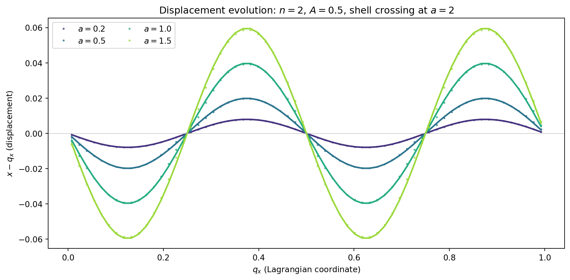
We compare the simulation output against the Zel’dovich prediction. Since the perturbation is along \(x\) only, we look at the \(x\)-displacement and \(x\)-momentum as functions of the Lagrangian coordinate \(q_x\).
fig, axes = plt.subplots(2, 1, figsize=(10, 7), sharex=True)

dx_sim = displacement(pos_final, q_grid, L)[slice_idx][sort_idx]
dx_exact = displacement(pos_exact, q_grid, L)[slice_idx][sort_idx]

# Momentum
px_sim = mom_final[slice_idx, 0][sort_idx]
px_exact = mom_exact[slice_idx, 0][sort_idx]

# --- Displacement ---
ax = axes[0]
ax.plot(q_x_sorted, dx_exact, '-', color='C1', lw=2, label='Zel\'dovich (exact)')
ax.plot(q_x_sorted, dx_sim, '.', color='C0', ms=3, alpha=0.7, label='PM simulation')
ax.set_ylabel('$x - q_x$ (displacement)')
ax.legend()
ax.set_title(f'Single sine wave: $n={n_mode}$, $A={A}$, '
             f'$a_i={a_init}$ → $a_f={a_final}$, {n_steps} steps')

# --- Momentum ---
ax = axes[1]
ax.plot(q_x_sorted, px_exact, '-', color='C1', lw=2, label='Zel\'dovich (exact)')
ax.plot(q_x_sorted, px_sim, '.', color='C0', ms=3, alpha=0.7, label='PM simulation')
ax.set_ylabel('$p_x$ (momentum)')
ax.set_xlabel('$q_x$ (Lagrangian coordinate)')
ax.legend()

plt.tight_layout()
plt.show()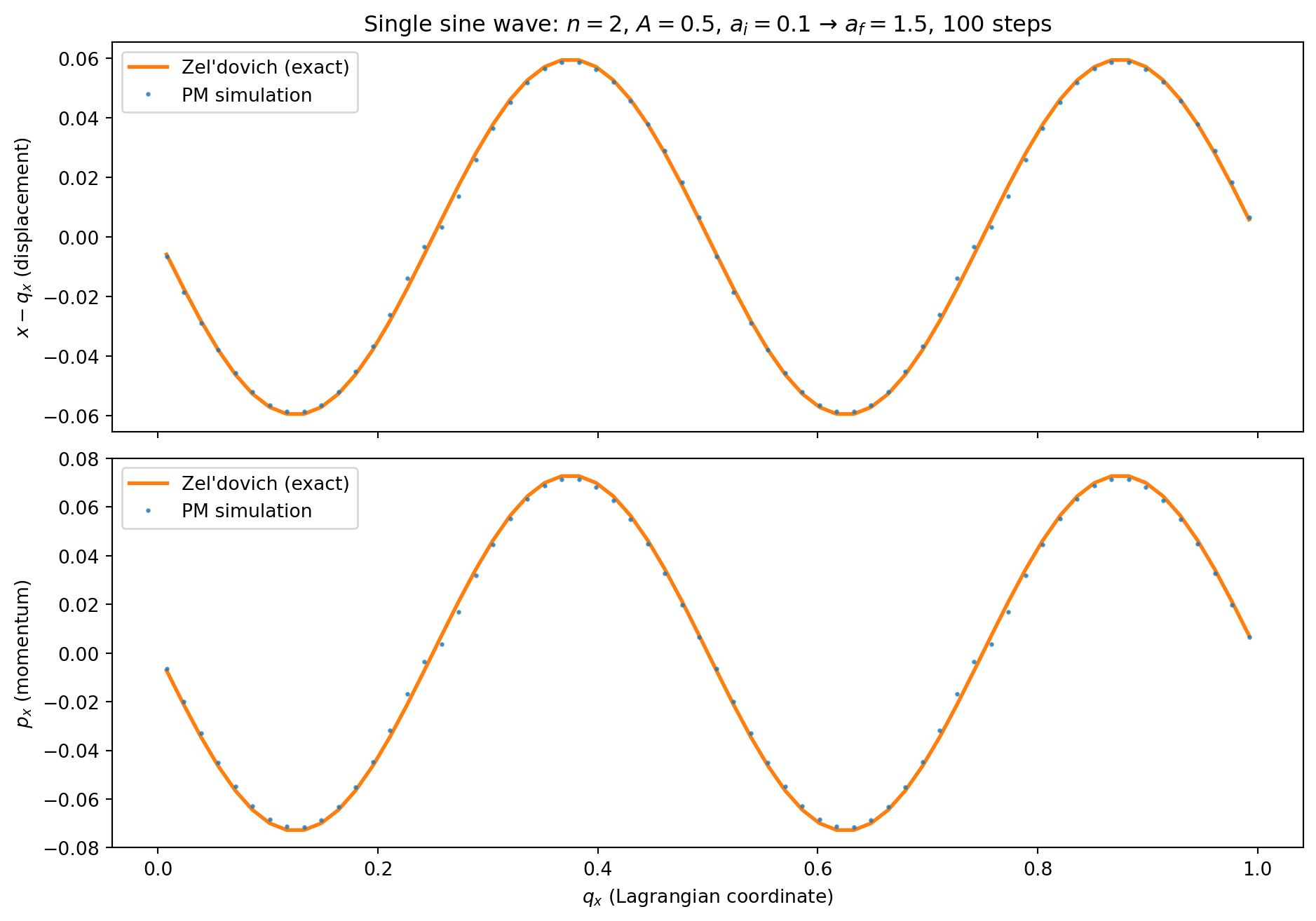
fig, axes = plt.subplots(2, 1, figsize=(10, 5), sharex=True)

dx_err = (dx_sim - dx_exact)
px_err = (px_sim - px_exact)

ax = axes[0]
ax.plot(q_x_sorted, dx_err, '.', color='C0', ms=3, alpha=0.7)
ax.axhline(0, color='0.5', lw=0.5)
ax.set_ylabel('$\\Delta(x - q_x)$')
ax.set_title('Absolute error relative to Zel\'dovich solution')

ax = axes[1]
ax.plot(q_x_sorted, px_err, '.', color='C0', ms=3, alpha=0.7)
ax.axhline(0, color='0.5', lw=0.5)
ax.set_ylabel('$\\Delta p_x$')
ax.set_xlabel('$q_x$ (Lagrangian coordinate)')

plt.tight_layout()
plt.show()

# Summary statistics
print(f"Displacement: max |error| = {jnp.max(jnp.abs(dx_err)):.2e}")
print(f"Momentum:     max |error| = {jnp.max(jnp.abs(px_err)):.2e}")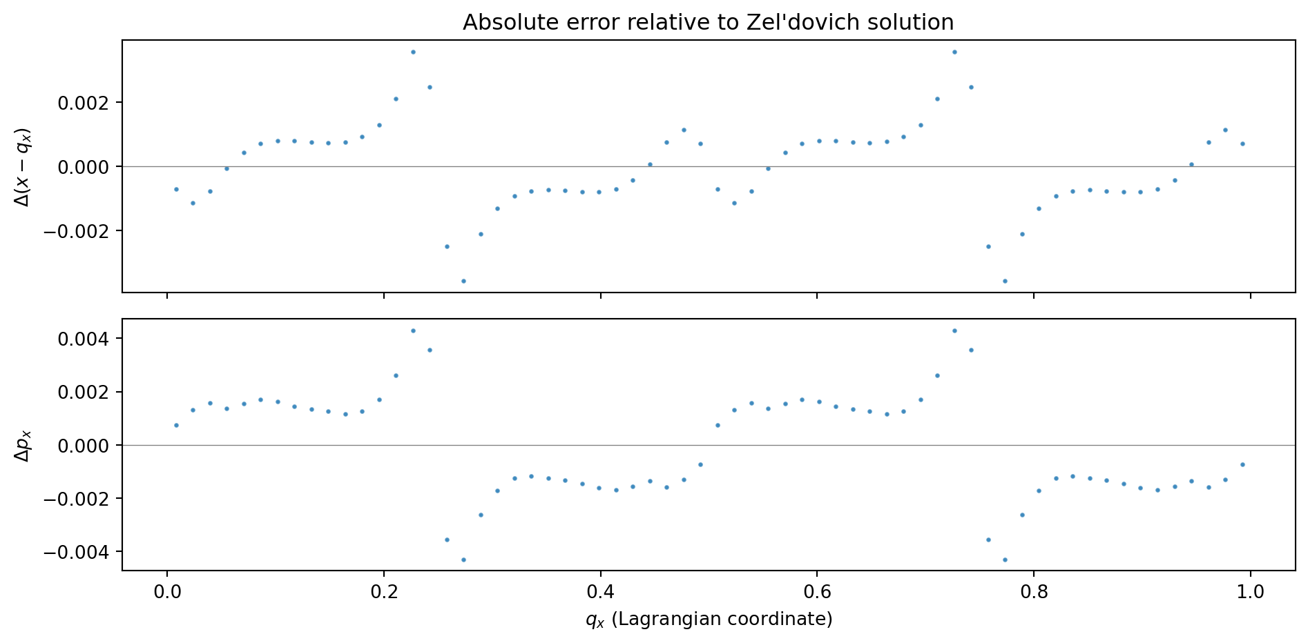
Displacement: max |error| = 3.58e-03
Momentum:     max |error| = 4.30e-03
The errors are at the \(\sim 10^{-3}\) level in both displacement and momentum. These errors have two sources: (1) time-stepping error from the KDK integrator, and (2) spatial error from the PM force calculation (CIC window function, discrete grid). We disentangle these below.
Let us verify the second-order convergence explicitly. A subtlety: if we compare against the exact Zel’dovich solution, the error is dominated by the spatial PM error (CIC window, discrete particle sampling) rather than the temporal error from the integrator. These spatial errors are independent of timestep count, creating a floor.
To isolate the time-stepping error, we compare each run against a high-resolution reference run (1000 steps) using the same PM code. The spatial errors cancel in the difference, leaving only the integrator error.
# High-resolution reference
pos_ref, mom_ref = run_simulation(
    pos_init, mom_init, a_init, a_final, 1000,
    green_x, green_y, green_z, Ng, L, Omega_m
)
dx_ref = displacement(pos_ref, q_grid, L)[slice_idx][sort_idx]
px_ref = mom_ref[slice_idx, 0][sort_idx]

step_counts = [5, 10, 20, 50, 100, 200]
dx_errors = []
px_errors = []

for ns in step_counts:
    pos_f, mom_f = run_simulation(
        pos_init, mom_init, a_init, a_final, ns,
        green_x, green_y, green_z, Ng, L, Omega_m
    )
    dx_s = displacement(pos_f, q_grid, L)[slice_idx][sort_idx]
    px_s = mom_f[slice_idx, 0][sort_idx]

    dx_errors.append(float(jnp.max(jnp.abs(dx_s - dx_ref))))
    px_errors.append(float(jnp.max(jnp.abs(px_s - px_ref))))

fig, ax = plt.subplots(1, 1, figsize=(8, 5))
ax.loglog(step_counts, dx_errors, 'o-', color='C0', label='max $|\\Delta x|$')
ax.loglog(step_counts, px_errors, 's-', color='C1', label='max $|\\Delta p_x|$')

# Reference line: N^{-2}
ns_ref = np.array(step_counts, dtype=float)
ax.loglog(ns_ref, dx_errors[0] * (ns_ref[0] / ns_ref)**2, '--',
          color='0.5', label='$\\propto N_{\\mathrm{steps}}^{-2}$')

ax.set_xlabel('Number of timesteps')
ax.set_ylabel('Maximum absolute error (vs 1000-step reference)')
ax.legend()
ax.set_title(f'Time-stepping convergence: mode $n={n_mode}$, $A={A}$, '
             f'$a: {a_init}$ → ${a_final}$')
plt.tight_layout()
plt.show()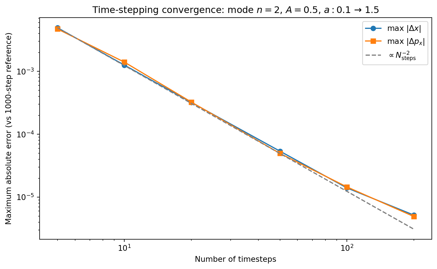
The timestep convergence test above isolates the integrator error by comparing against a reference run with the same spatial resolution. But how large is the spatial PM error itself? We can test this by running the same problem at increasing grid resolution \(N_g = N_p\) (keeping 1 particle per cell and using enough timesteps that the time-stepping error is negligible) and comparing against the exact Zel’dovich solution.
grid_sizes = [32, 64, 128]
n_steps_hires = 500  # enough steps to make time-stepping error negligible

dx_spatial_errors = []
px_spatial_errors = []

for N in grid_sizes:
    # Set up at this resolution
    green_xi, green_yi, green_zi = make_green_function(N, L)
    pos_i, mom_i, q_i = make_zeldovich_ic(N, L, n_mode, A, a_init)
    slice_i = jnp.arange(0, N**3, N**2)

    # Run simulation
    pos_f, mom_f = run_simulation(
        pos_i, mom_i, a_init, a_final, n_steps_hires,
        green_xi, green_yi, green_zi, N, L, Omega_m
    )

    # Exact solution
    pos_e, mom_e = zeldovich_prediction(q_i, n_mode, A, a_final, L)

    # Errors on the 1D slice
    q_xi = q_i[slice_i, 0]
    sort_i = jnp.argsort(q_xi)

    dx_f = displacement(pos_f, q_i, L)[slice_i][sort_i]
    dx_e = displacement(pos_e, q_i, L)[slice_i][sort_i]
    px_f = mom_f[slice_i, 0][sort_i]
    px_e = mom_e[slice_i, 0][sort_i]

    dx_spatial_errors.append(float(jnp.max(jnp.abs(dx_f - dx_e))))
    px_spatial_errors.append(float(jnp.max(jnp.abs(px_f - px_e))))

    print(f"Ng=Np={N:3d}: max |Δx| = {dx_spatial_errors[-1]:.2e}, "
          f"max |Δp| = {px_spatial_errors[-1]:.2e}")

fig, ax = plt.subplots(1, 1, figsize=(8, 5))
ax.loglog(grid_sizes, dx_spatial_errors, 'o-', color='C0',
          label='max $|\\Delta x|$')
ax.loglog(grid_sizes, px_spatial_errors, 's-', color='C1',
          label='max $|\\Delta p_x|$')

# Reference line: N^{-1}
ns_ref = np.array(grid_sizes, dtype=float)
ax.loglog(ns_ref, dx_spatial_errors[0] * (ns_ref[0] / ns_ref)**1, '--',
          color='0.5', label='$\\propto N_g^{-1}$')

ax.set_xlabel('Grid size $N_g = N_p$')
ax.set_ylabel('Maximum absolute error (vs exact Zel\'dovich)')
ax.legend()
ax.set_title(f'Spatial convergence: mode $n={n_mode}$, $A={A}$, '
             f'$a: {a_init}$ → ${a_final}$, {n_steps_hires} steps')
plt.tight_layout()
plt.show()
Ng=Np= 32: max |Δx| = 7.50e-03, max |Δp| = 9.23e-03
Ng=Np= 64: max |Δx| = 3.58e-03, max |Δp| = 4.30e-03
Ng=Np=128: max |Δx| = 1.77e-03, max |Δp| = 2.11e-03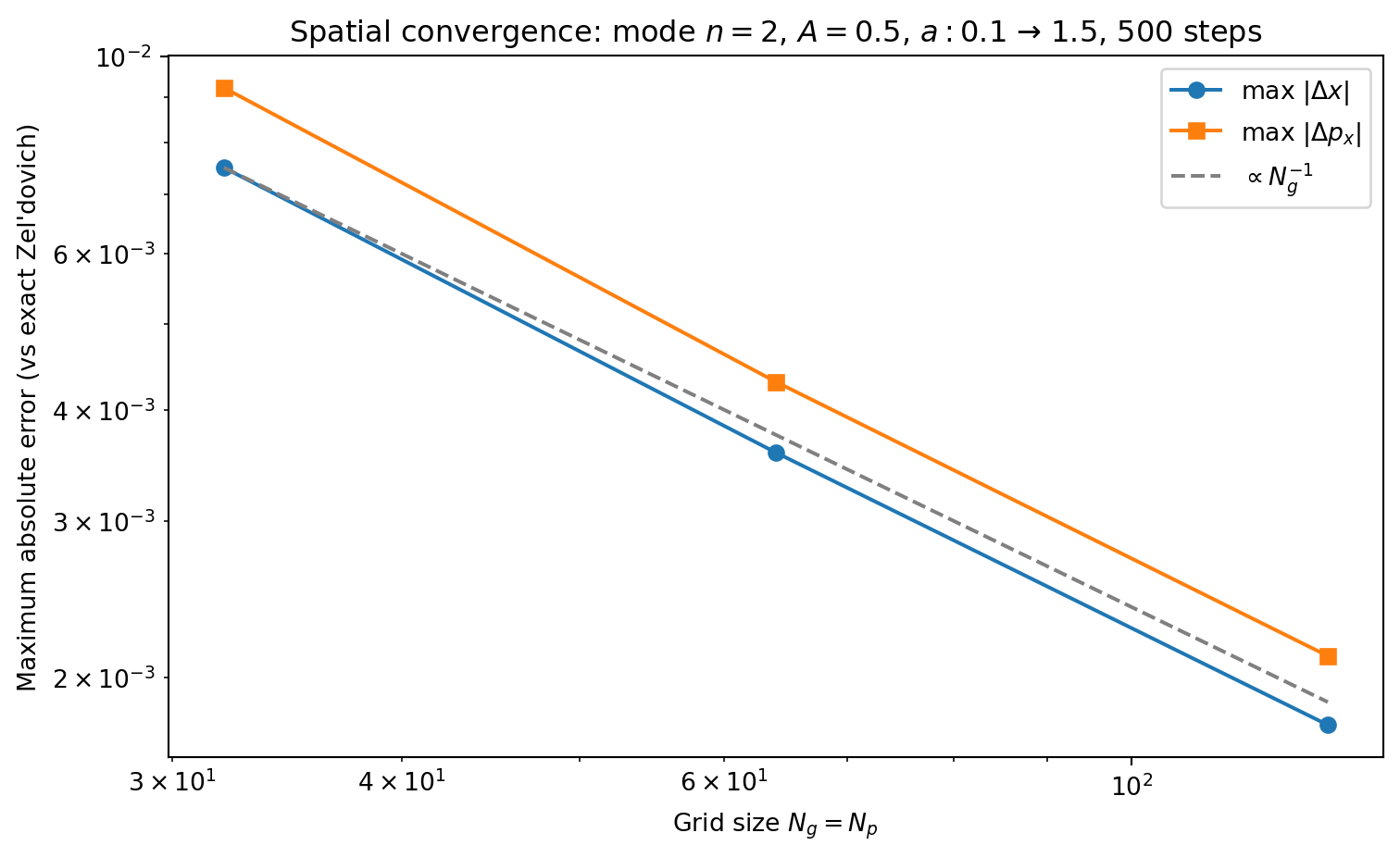
The spatial error decreases as \(\sim N_g^{-1}\), not \(N_g^{-2}\). This may seem surprising since the discrete gradient and Laplacian operators are both second-order accurate. The bottleneck is CIC itself: CIC is a first-order (piecewise linear) interpolation scheme, producing a density field that is \(C^0\) but not \(C^1\). The resulting force — the gradient of the potential — is discontinuous at cell boundaries, with \(\mathcal{O}(h)\) jumps. This limits the maximum force error at particle positions to \(\mathcal{O}(h) = \mathcal{O}(N_g^{-1})\), regardless of how accurate the Poisson solver is.
Higher-order mass assignment schemes improve this: TSC (second-order B-spline) gives continuous forces and \(\mathcal{O}(N_g^{-2})\) spatial convergence.
We now put the pieces together and run a cosmological simulation with realistic initial conditions drawn from the matter power spectrum.
To generate cosmological ICs we need:
from classy import Class

# Set up CLASS with Planck-like cosmology
cosmo = Class()
cosmo.set({
    'output': 'mPk',
    'h': 0.7,
    'omega_b': 0.02237,
    'omega_cdm': 0.1200,
    'A_s': 2.1e-9,
    'n_s': 0.9649,
    'P_k_max_h/Mpc': 50.0,
    'z_max_pk': 100.0
})
cosmo.compute()

h_class = cosmo.h()
print(f"CLASS cosmology: Omega_m = {cosmo.Omega_m():.4f}, "
      f"h = {h_class:.3f}, sigma8 = {cosmo.sigma8():.4f}")
CLASS cosmology: Omega_m = 0.2906, h = 0.700, sigma8 = 0.8300Our PM code uses Einstein–de Sitter dynamics (\(\Omega_m = 1\)). We use the CLASS power spectrum for the shape of \(P(k)\) (which encodes the transfer function, BAO, etc.) but evolve under EdS gravity. This is a common simplification in pedagogical codes — the large-scale structure looks qualitatively correct, but the growth rate and normalization differ from \(\Lambda\)CDM. A production code would use the correct \(H(a)\) and growth factor for the target cosmology.
# Simulation parameters for cosmological run
Ng_cosmo = 128
Np_cosmo = 128
L_cosmo = 200.0       # Mpc/h (comoving box size)
z_init = 49.0
a_init_cosmo = 1.0 / (1.0 + z_init)

# Build the P(k) interpolator at z=0.
# The Zel'dovich displacement field Psi is defined via delta_0 (the
# present-day density), so we need P(k, z=0). The growth factor D_+(a)
# then scales the displacement to the initial time.
k_arr = np.logspace(-4, np.log10(50.0), 2000)  # k in h/Mpc
pk_arr = np.array([cosmo.pk(k * h_class, 0.0) * h_class**3
                   for k in k_arr])  # P(k, z=0) in (Mpc/h)^3

# Clean up CLASS
cosmo.struct_cleanup()

# Interpolate in log-log space
from scipy.interpolate import interp1d
log_pk_interp = interp1d(np.log(k_arr), np.log(pk_arr),
                         kind='cubic', fill_value=-100.0,
                         bounds_error=False)

def pk_of_k(k):
    """P(k) in (Mpc/h)^3, k in h/Mpc."""
    return np.exp(log_pk_interp(np.log(k)))

print(f"Box: L = {L_cosmo} Mpc/h, Ng = Np = {Ng_cosmo}")
print(f"Starting at z = {z_init} (a = {a_init_cosmo:.4f})")
print(f"Fundamental mode: k_f = {2*np.pi/L_cosmo:.4f} h/Mpc")
print(f"Nyquist: k_Ny = {np.pi*Ng_cosmo/L_cosmo:.2f} h/Mpc")
Box: L = 200.0 Mpc/h, Ng = Np = 128
Starting at z = 49.0 (a = 0.0200)
Fundamental mode: k_f = 0.0314 h/Mpc
Nyquist: k_Ny = 2.01 h/Mpcdef make_cosmo_ic(Np, Ng, L, pk_func, a_init, seed=42):
"""
Generate cosmological Zel'dovich ICs from a power spectrum.
Parameters
----------
Np : int
Particles per dimension.
Ng : int
Grid cells per dimension.
L : float
Box size (same units as P(k), e.g. Mpc/h).
pk_func : callable
P(k) function, k in h/Mpc, returns (Mpc/h)^3.
a_init : float
Initial scale factor.
seed : int
Random seed.
Returns
-------
pos, mom, q : arrays
Positions, momenta, and Lagrangian grid.
"""
h = L / Ng
V = L**3
# Wavenumber grid (angular wavenumber k in h/Mpc)
# fftfreq returns frequency nu = n/(N*h); multiply by 2pi for k
kfreq = 2 * np.pi * np.fft.fftfreq(Ng, d=h) # k in h/Mpc
kx, ky, kz = np.meshgrid(kfreq, kfreq, kfreq, indexing='ij')
kmag = np.sqrt(kx**2 + ky**2 + kz**2)
kmag[0, 0, 0] = 1.0 # avoid division by zero
# Power spectrum on the grid
pk_grid = pk_func(kmag)
pk_grid[0, 0, 0] = 0.0 # no mean overdensity
# Generate Gaussian random field by "coloring" white noise.
# Start with real-space white noise, FFT it (reality condition is
# automatic since the input is real), then multiply by sqrt(P(k))
# to imprint the power spectrum.
#
# Normalization: E[|noise_hat_k|^2] = Ng^3 for white noise.
# We want E[|delta_hat_k|^2] = Ng^6 P(k) / V, so multiply
# noise_hat by Ng^{3/2} sqrt(P(k)/V).
rng = np.random.default_rng(seed)
white_noise = rng.standard_normal((Ng, Ng, Ng))
noise_hat = np.fft.fftn(white_noise)
amplitude = Ng**1.5 * np.sqrt(pk_grid / V)
delta_hat = amplitude * noise_hat
delta_hat[0, 0, 0] = 0.0 # no mean overdensity
# Displacement field: Psi_i(k) = -i k_i / k^2 * delta_hat(k)
inv_k2 = 1.0 / (kmag**2)
inv_k2[0, 0, 0] = 0.0
psi_hat_x = -1j * kx * inv_k2 * delta_hat
psi_hat_y = -1j * ky * inv_k2 * delta_hat
psi_hat_z = -1j * kz * inv_k2 * delta_hat
# Transform to real space
psi_x = np.fft.ifftn(psi_hat_x).real
psi_y = np.fft.ifftn(psi_hat_y).real
psi_z = np.fft.ifftn(psi_hat_z).real
# Lagrangian grid
q = make_uniform_grid(Np, L)
q_np = np.array(q)
# Interpolate displacement to particle positions
# For Np = Ng, particles sit at grid centers — direct indexing
idx = np.round(q_np / h - 0.5).astype(int) % Ng
psi_at_q = np.stack([
psi_x[idx[:, 0], idx[:, 1], idx[:, 2]],
psi_y[idx[:, 0], idx[:, 1], idx[:, 2]],
psi_z[idx[:, 0], idx[:, 1], idx[:, 2]],
], axis=-1)
# Zel'dovich: x = q + D_+(a) * Psi, p = a^{3/2} * Psi (EdS)
pos = jnp.array((q_np + a_init * psi_at_q) % L)
mom = jnp.array(a_init**1.5 * psi_at_q)
return pos, mom, q
pos_cosmo, mom_cosmo, q_cosmo = make_cosmo_ic(
Np_cosmo, Ng_cosmo, L_cosmo, pk_of_k, a_init_cosmo
)
print(f"Particles: {pos_cosmo.shape[0]:,}")
print(f"Initial rms displacement: {np.std(np.array(pos_cosmo - q_cosmo)):.4f} Mpc/h")Particles: 2,097,152
Initial rms displacement: 0.1098 Mpc/h# Precompute Green's function for the cosmological grid
green_cx, green_cy, green_cz = make_green_function(Ng_cosmo, L_cosmo)
# Run from z=49 to z=0 (a=0.02 to a=1)
a_final_cosmo = 1.0
n_steps_cosmo = 100
print(f"Running {Np_cosmo}^3 simulation: a = {a_init_cosmo:.4f} → {a_final_cosmo}")
print(f" {n_steps_cosmo} steps, Ng = {Ng_cosmo}, L = {L_cosmo} Mpc/h")
pos_cosmo_final, mom_cosmo_final = run_simulation(
pos_cosmo, mom_cosmo, a_init_cosmo, a_final_cosmo, n_steps_cosmo,
green_cx, green_cy, green_cz, Ng_cosmo, L_cosmo, 1.0
)
print("Done!")Running 128^3 simulation: a = 0.0200 → 1.0
100 steps, Ng = 128, L = 200.0 Mpc/h
Done!We visualize the result by depositing particles onto the grid and showing a thin slice through the density field.
# Deposit final positions onto grid
rho_final = cic_deposit(pos_cosmo_final, Ng_cosmo, L_cosmo)
rho_bar = Np_cosmo**3 / Ng_cosmo**3
delta_final = rho_final / rho_bar - 1.0

# Take a thin slice (single grid plane)
slice_z = Ng_cosmo // 2

fig, ax = plt.subplots(1, 1, figsize=(8, 8))

im = ax.imshow(
    np.log10(np.maximum(1 + np.array(delta_final[:, :, slice_z]), 1e-6)).T,
    origin='lower',
    extent=[0, L_cosmo, 0, L_cosmo],
    cmap='magma',
    vmin=-0.5,
    vmax=2.0
)
ax.set_xlabel('$x$ [Mpc/$h$]')
ax.set_ylabel('$y$ [Mpc/$h$]')
ax.set_title(f'$z = 0$ density slice ($N_g = {Ng_cosmo}$, '
             f'$L = {L_cosmo}$ Mpc/$h$)')
plt.colorbar(im, ax=ax, label='$\\log_{10}(1 + \\delta)$', shrink=0.8)
plt.tight_layout()
plt.show()

# Statistics
print(f"Density field statistics at z=0:")
print(f"  min(delta) = {delta_final.min():.2f}")
print(f"  max(delta) = {delta_final.max():.1f}")
print(f"  rms(delta) = {jnp.std(delta_final):.2f}")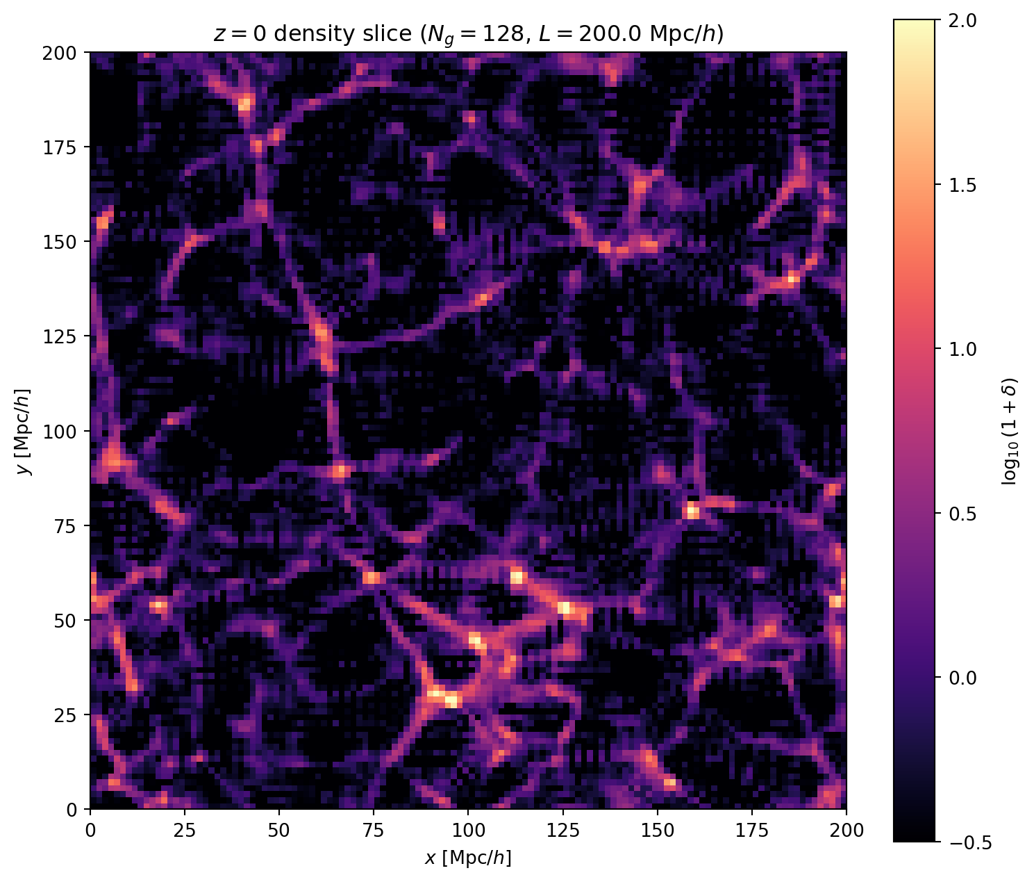
Density field statistics at z=0:
  min(delta) = -1.00
  max(delta) = 494.1
rms(delta) = 3.68a_snaps = [0.1, 0.2, 0.5, 1.0]
z_snaps = [1/a - 1 for a in a_snaps]
fig, axes = plt.subplots(1, 4, figsize=(18, 4.5),
gridspec_kw={'wspace': 0.05, 'right': 0.92})
for ax, a_snap, z_snap in zip(axes, a_snaps, z_snaps):
pos_s, _ = run_simulation(
pos_cosmo, mom_cosmo, a_init_cosmo, a_snap, n_steps_cosmo,
green_cx, green_cy, green_cz, Ng_cosmo, L_cosmo, 1.0
)
rho_s = cic_deposit(pos_s, Ng_cosmo, L_cosmo)
delta_s = rho_s / rho_bar - 1.0
im = ax.imshow(
np.log10(np.maximum(1 + np.array(delta_s[:, :, slice_z]), 1e-6)).T,
origin='lower',
extent=[0, L_cosmo, 0, L_cosmo],
cmap='magma',
vmin=-0.5,
vmax=2.0
)
ax.set_title(f'$z = {z_snap:.0f}$')
ax.set_xlabel('$x$ [Mpc/$h$]')
if ax == axes[0]:
ax.set_ylabel('$y$ [Mpc/$h$]')
else:
ax.set_yticklabels([])
ax.set_aspect('equal')
cbar_ax = fig.add_axes([0.93, 0.15, 0.015, 0.7])
fig.colorbar(im, cax=cbar_ax, label='$\\log_{10}(1 + \\delta)$')
plt.show()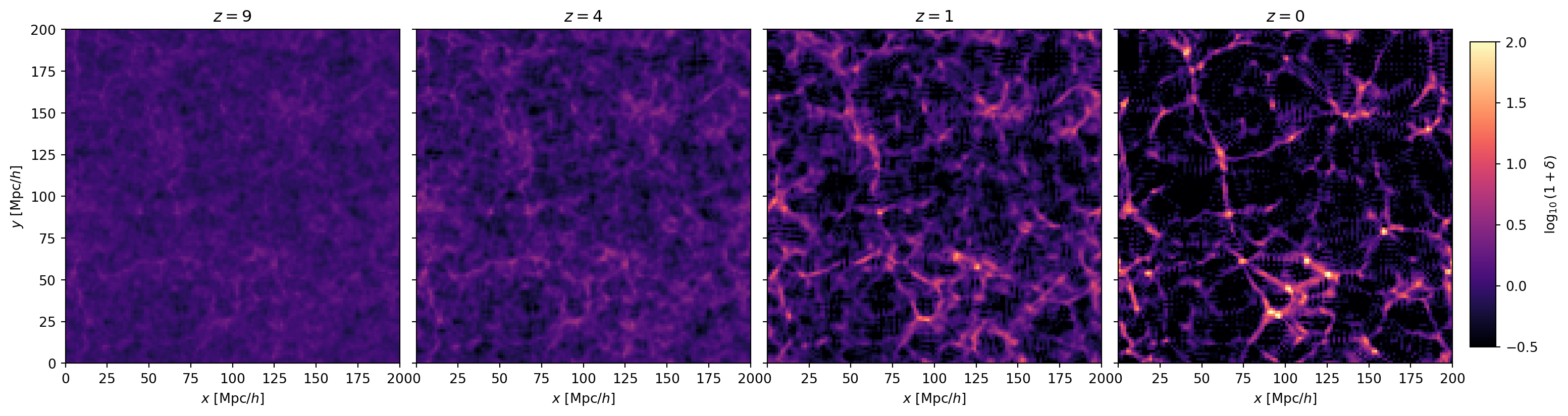
Finally, let us watch the cosmic web form in real time. We run the simulation to 50 intermediate epochs and assemble the density slices into a movie.
from matplotlib.animation import FuncAnimation
from IPython.display import Video

# Scale factors for the movie frames (log-spaced)
n_frames = 50
a_frames = np.exp(np.linspace(np.log(a_init_cosmo), np.log(a_final_cosmo), n_frames))

# Run simulation to each epoch and store density slices
slices = []
for a_snap in a_frames:
    n_steps_snap = max(10, int(100 * (a_snap - a_init_cosmo) / (a_final_cosmo - a_init_cosmo)))
    pos_s, _ = run_simulation(
        pos_cosmo, mom_cosmo, a_init_cosmo, a_snap, n_steps_snap,
        green_cx, green_cy, green_cz, Ng_cosmo, L_cosmo, 1.0
    )
    rho_s = cic_deposit(pos_s, Ng_cosmo, L_cosmo)
    delta_s = rho_s / rho_bar - 1.0
    slices.append(
        np.log10(np.maximum(1 + np.array(delta_s[:, :, slice_z]), 1e-6)).T
    )

# Build animation
fig, ax = plt.subplots(1, 1, figsize=(7, 7))
im = ax.imshow(slices[0], origin='lower',
               extent=[0, L_cosmo, 0, L_cosmo],
               cmap='magma', vmin=-0.5, vmax=2.0)
ax.set_xlabel('$x$ [Mpc/$h$]')
ax.set_ylabel('$y$ [Mpc/$h$]')
title = ax.set_title(f'$z = {1/a_frames[0] - 1:.1f}$')
fig.colorbar(im, ax=ax, label='$\\log_{10}(1 + \\delta)$', shrink=0.8)
fig.tight_layout()

def update(frame):
    im.set_data(slices[frame])
    z_val = 1/a_frames[frame] - 1
    title.set_text(f'$z = {z_val:.1f}$')
    return [im, title]

anim = FuncAnimation(fig, update, frames=n_frames, interval=150, blit=True)

# Save as MP4
movie_path = 'cosmic_web_evolution.mp4'
anim.save(movie_path, writer='ffmpeg', dpi=120)
plt.close(fig)

Video(movie_path, embed=True, html_attributes='controls loop autoplay muted width="700"')This is the cosmic web emerging from nearly uniform initial conditions through gravitational instability alone — no hydrodynamics, no star formation, just dark matter and gravity computed on a \(128^3\) grid with the PM algorithm we built from scratch in this lecture.