1 Trajectories in an Expanding Universe
We now consider the trajectories of free particles in an expanding Universe. The most direct and global treatment of this comes by deriving the geodesic equation, which all particles follow. However, one can get interesting intuition by considering local patches (where special relativity is valid), and stitching these together. We consider three such variants below.
1.1 Photons
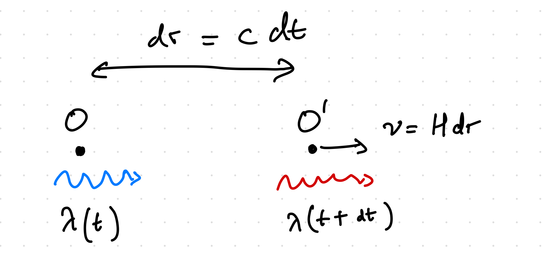
(This treatment is essentially the same as our derivation of the connection between redshift and the scale factor, although the apparent presentation looks different) Consider a photon emitted by O at time \(t\), and detected by a second observer O’ at time \(t+dt\). This second observer is therefore a distance \(c dt\) away, and must be receding with a velocity of \(H c dt\) by Hubble’s law. The doppler shift of the photon is therefore \[ \frac{\lambda(t+dt)}{\lambda(t)} = \sqrt{\frac{1+v}{1-v}} \] where, for simplicity, we now just use \(c=1\). Since we are assuming infinitesimal intervals, we can Taylor expand both sides to get \[ \frac{\dot{\lambda}\,dt}{\lambda} = v = H\,dt = \frac{\dot{a}}{a} dt \] from which we get \[ \frac{d\lambda}{\lambda} = \frac{d a}{a} \] or \[ \lambda \propto a \] This is just the definition of redshift, rewritten. Since the momentum and energy of a photon is inversely proportional to its wavelength, this implies \[ E \propto p \propto \frac{1}{a} \] or that photons lose energy in an expanding Universe.
1.2 Momentum Decay
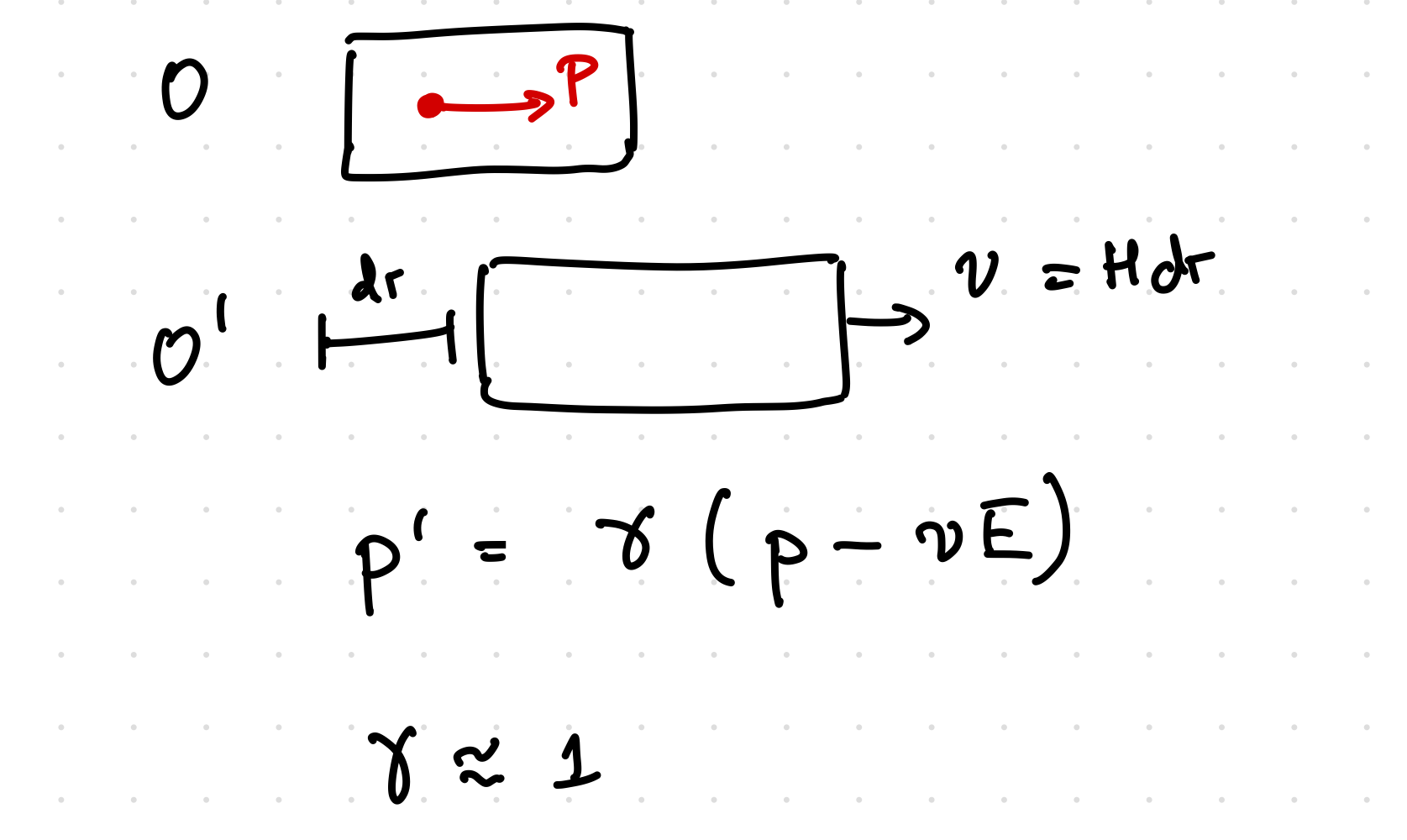 The figure above sets up the two frames that we want to consider. As before, we consider these to be almost coincident, so that the velocity is very small and \(\gamma \approx 1\). Writing down the Lorentz transformation between the two frames, we have \[
p’ = \gamma (p - v E)
\] In our limit, this yields \[
\begin{aligned}
dp & \approx -v E \\
& = - (H \, dr) E \\
& = - \frac{\dot{a}}{a} (u \,dt) E \\
& = - \frac{\dot{a}}{a} (\frac{p}{E} \,dt) E
\end{aligned}
\] where we used the fact that \(dr = u \,dt\) with \(u\) being the velocity corresponding to the momentum \(p\), and then, \(u = p/E\) which is true in both the massless and massive regimes. Putting this all together, we get \[
\frac{dp}{p} = - \frac{da}{a}
\] or \[
p \propto \frac{1}{a}
\] Again, this is a statement that energy/momentum decays away in an expanding Universe. In the case of massive particles, this is purely a simple kinematic effect, with the particle needing to “catch up” with a series of receding observers.
The figure above sets up the two frames that we want to consider. As before, we consider these to be almost coincident, so that the velocity is very small and \(\gamma \approx 1\). Writing down the Lorentz transformation between the two frames, we have \[
p’ = \gamma (p - v E)
\] In our limit, this yields \[
\begin{aligned}
dp & \approx -v E \\
& = - (H \, dr) E \\
& = - \frac{\dot{a}}{a} (u \,dt) E \\
& = - \frac{\dot{a}}{a} (\frac{p}{E} \,dt) E
\end{aligned}
\] where we used the fact that \(dr = u \,dt\) with \(u\) being the velocity corresponding to the momentum \(p\), and then, \(u = p/E\) which is true in both the massless and massive regimes. Putting this all together, we get \[
\frac{dp}{p} = - \frac{da}{a}
\] or \[
p \propto \frac{1}{a}
\] Again, this is a statement that energy/momentum decays away in an expanding Universe. In the case of massive particles, this is purely a simple kinematic effect, with the particle needing to “catch up” with a series of receding observers.
1.3 A Lagrangian Approach
We consider a third approach, using a Lagrangian. Recall \[S = -m \int ds \quad \leftarrow \text{Lorentz invariant}\] which, if we limit to one spatial dimension gives us \[= -m \int \left[ 1 - a(t)^2 \left(\frac{dx}{dt}\right)^2 \right]^{1/2} dt \quad \leftarrow \text{1D motion}\] from where we can read off the Lagrangian. \[\mathcal{L} = -m \left[ 1 - a(t)^2 \left(\frac{dx}{dt}\right)^2 \right]^{1/2}\] We can now compute the conjugate momentum \[p = \frac{\partial \mathcal{L}}{\partial \dot{x}} \quad \leftarrow \text{conjugate momentum}\] \[\Rightarrow p = m \frac{1}{\left[ 1 - a(t)^2 \left(\frac{dx}{dt}\right)^2 \right]^{1/2}} a^2 \dot{x}\] We also observe that \(p\) is conserved. We can now solve for \(\dot{x}\) \[p^2 \left(1 - a^2 \dot{x}^2 \right) = m^2 a^4 \dot{x}^2\] \[\dot{x}^2 = \frac{p^2}{a^2 \left(p^2 + m^2 a^2\right)}\] Let us consider the cases of a massless and very massive (non-relativistic) particle.
\(m = 0\)
\[\begin{aligned} \dot{x} &\propto \frac{1}{a} \\ v_{\text{pec}} &\sim a \dot{x} \\ &\sim \text{constant as expected for massless} \end{aligned}\]
\(m \gg p\)
\[\begin{aligned} \dot{x} &\propto \frac{1}{a^2} \\ v_{\text{pec}} &\propto \frac{1}{a} \quad \leftarrow \text{same as before.} \end{aligned}\]