Code
import numpy as np
import matplotlib.pyplot as plt
import os.path

# Define path to data
# You will need to adjust this on the cluster
DATA_DIR = os.path.expanduser("~/data/teaching/ASTR6000-SP26")Our goal in this notebook is to compute and plot the Quijote mass function.
You can find the details of the Quijote simulations here.
We are using a subset of the Quijote simulations for this analysis; these will be made available on the cluster (the directory will be shared separately). The notebook here uses a directory structure set up on my laptop/desktop, so you will need to adjust these if you want to run this notebook.
import numpy as np
import matplotlib.pyplot as plt
import os.path
# Define path to data
# You will need to adjust this on the cluster
DATA_DIR = os.path.expanduser("~/data/teaching/ASTR6000-SP26")Unlike our previous analyses of the power spectra, we will need to actually load and process the halo catalogs. These are stored as binary files in the Quijote data directory, and so, we will use a simple helper function to read these in (for now, we’ll just need the halo masses).
The halo catalogs are organized by simulation number and snapshot number, where the snapshot number corresponds to different redshifts. In the Quijote simulations, snapshot 4 corresponds to \(z=0\).
def read_quijote_masses(sim_num, snap_num=4):
    """Reads halo masses from Quijote FoF binary without Pylians."""
    file_path = os.path.join(DATA_DIR, f"Quijote-Halos-HR/{sim_num}/group_tab_{snap_num:03d}.0")
    print(f"Reading halo catalog from {file_path}")


    with open(file_path, 'rb') as f:
        # Read Header: 8 integers (N_groups, N_tot, N_ids, Tot_N_ids, etc.)
        header = np.fromfile(f, dtype=np.int32, count=6)
        ngroups = header[0]

        # Validate
        if ngroups != header[1]:
            raise ValueError("N_groups does not match N_tot in header, as expected for a single file!")
        if ngroups < 1:
            raise ValueError("No groups found in the file!")
        if header[5] != 1:
            print(f"Unexpected header: {header}")
            raise ValueError("This function only supports single file catalogs (not split across multiple files).")

        print(f"Number of groups in file: {ngroups}")

        # Skip first two arrays
        np.fromfile(f, dtype=np.int32, count=ngroups)  # Group offsets
        np.fromfile(f, dtype=np.int32, count=ngroups)  # Group lengths
        # Read masses
        # Masses are stored as float32 in units of 1e10 M_sun/h
        masses = np.fromfile(f, dtype=np.float32, count=ngroups)

        masses *= 1e10  # Convert to M_sun/h

        print(f"Read {len(masses)} halo masses. Min mass: {masses.min():.2e} M_sun/h, Max mass: {masses.max():.2e} M_sun/h")

return masses # Test the function by reading masses from simulation 0, snapshot 4
masses = read_quijote_masses(sim_num=0, snap_num=4)Reading halo catalog from /Users/npadmana/data/teaching/ASTR6000-SP26/Quijote-Halos-HR/0/group_tab_004.0
Number of groups in file: 2946947
Read 2946947 halo masses. Min mass: 1.64e+12 M_sun/h, Max mass: 5.38e+15 M_sun/hThe mass function is nothing but a histogram of halo masses. Let us set up the mass bins so that we can accumulate the halo mass functions for multiple simulations. We’ll use logarithmic bins from \(5 \times 10^{12}\) to \(5 \times 10^{15}\,M_\odot/h\) with 30 bins in total.
We’ll test this out for a single simulation first.
Finally, we’ll define overall normalizations, including the volume and the bin widths, so that what we get is dn/dlnM in units of (Mpc/h)\(^{-3}\).
mass_bins = np.linspace(np.log10(5e12), np.log10(5e15), 31)

# Test histogram for a single simulation
hist, bin_edges = np.histogram(np.log10(masses), bins=mass_bins)
print("Mass bin edges (log10 M_sun/h):", bin_edges)
print("Mass function (counts per bin):", hist)

Lbox = 1000.0  # Mpc/h
bin_widths = np.diff(bin_edges)  # in log10(M_sun/h)
volume = Lbox**3  # (Mpc/h)^3
normalization = 1.0 / (volume * bin_widths * np.log(10))  # Convert from log10 to ln
Mass bin edges (log10 M_sun/h): [12.69897 12.79897 12.89897 12.99897 13.09897 13.19897 13.29897 13.39897
13.49897 13.59897 13.69897 13.79897 13.89897 13.99897 14.09897 14.19897
14.29897 14.39897 14.49897 14.59897 14.69897 14.79897 14.89897 14.99897
15.09897 15.19897 15.29897 15.39897 15.49897 15.59897 15.69897]
Mass function (counts per bin): [207251 165954 133980 109590 86609 70920 56822 45131 35736 28671
22181 17621 13443 10425 7755 5786 4203 2987 2137 1404
932 546 357 191 123 40 18 9 4 0]We can now compute and plot the mass function for the first 5 Quijote simulations. We’ll plot the individual mass functions, but also the average mass function.
sim_numbers = range(5)

mass_functions = []
for sim_num in sim_numbers:
    masses = read_quijote_masses(sim_num=sim_num, snap_num=4)
    hist, _ = np.histogram(np.log10(masses), bins=mass_bins)
    dndlnM = hist * normalization
    mass_functions.append(dndlnM)

mass_functions = np.array(mass_functions)
mean_mass_function = mass_functions.mean(axis=0)

bin_centers_log10 = 0.5 * (bin_edges[:-1] + bin_edges[1:])
mass_centers = 10**bin_centers_log10

plt.figure(figsize=(7, 5))
for dndlnM in mass_functions:
    mask = dndlnM > 0
    plt.plot(mass_centers[mask], dndlnM[mask], color='0.7', lw=1.0)

mean_mask = mean_mass_function > 0
plt.plot(
    mass_centers[mean_mask],
    mean_mass_function[mean_mask],
    color='k',
    lw=2.5,
    label='Mean (5 sims)',
)

plt.xscale('log')
plt.yscale('log')
plt.xlabel(r"$M\,[M_\odot/h]$")
plt.ylabel(r"$\mathrm{d}n/\mathrm{d}\ln M\;[(\mathrm{Mpc}/h)^{-3}]$")
plt.title("Quijote Halo Mass Function at $z=0$")
plt.legend()
plt.grid(alpha=0.3)
plt.tight_layout()
plt.show()
Reading halo catalog from /Users/npadmana/data/teaching/ASTR6000-SP26/Quijote-Halos-HR/0/group_tab_004.0
Number of groups in file: 2946947
Read 2946947 halo masses. Min mass: 1.64e+12 M_sun/h, Max mass: 5.38e+15 M_sun/h
Reading halo catalog from /Users/npadmana/data/teaching/ASTR6000-SP26/Quijote-Halos-HR/1/group_tab_004.0
Number of groups in file: 2946445
Read 2946445 halo masses. Min mass: 1.64e+12 M_sun/h, Max mass: 3.97e+15 M_sun/h
Reading halo catalog from /Users/npadmana/data/teaching/ASTR6000-SP26/Quijote-Halos-HR/2/group_tab_004.0
Number of groups in file: 2945544
Read 2945544 halo masses. Min mass: 1.64e+12 M_sun/h, Max mass: 4.39e+15 M_sun/h
Reading halo catalog from /Users/npadmana/data/teaching/ASTR6000-SP26/Quijote-Halos-HR/3/group_tab_004.0
Number of groups in file: 2945565
Read 2945565 halo masses. Min mass: 1.64e+12 M_sun/h, Max mass: 4.01e+15 M_sun/h
Reading halo catalog from /Users/npadmana/data/teaching/ASTR6000-SP26/Quijote-Halos-HR/4/group_tab_004.0
Number of groups in file: 2945565
Read 2945565 halo masses. Min mass: 1.64e+12 M_sun/h, Max mass: 4.01e+15 M_sun/h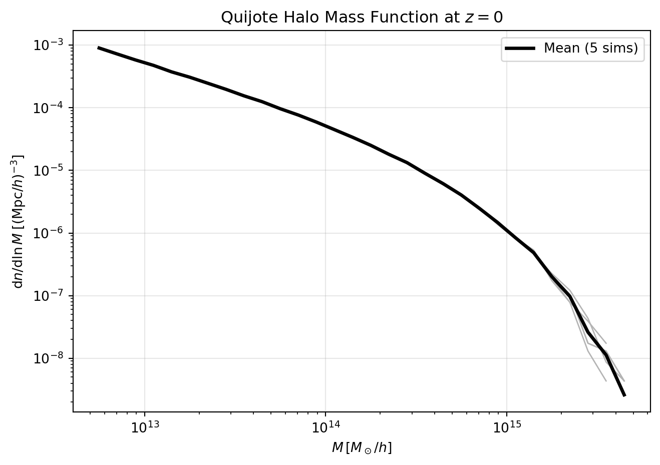
We can compare these results to the Press-Schechter mass function. Recall that the Press-Schechter mass function is given by:
\[ \frac{\mathrm{d}n}{\mathrm{d}\ln M} = \sqrt{\frac{2}{\pi}} \frac{\bar{\rho}}{M} \nu e^{-\nu^2/2} \left| \frac{\mathrm{d}\ln \sigma}{\mathrm{d}\ln M} \right| \] where \(\nu = \delta_c / \sigma(M)\), \(\delta_c \approx 1.686\), and \(\sigma(M)\) is the variance of the linear density field smoothed on scale \(M\).
There are a few steps to compute this:
Let’s go through these steps one by one.
# Load the linear theory power spectrum
linear_pk_file = os.path.join(DATA_DIR, "Quijote-Pk", "CAMB_matterpow_0.dat")
k_linear, pk_linear = np.loadtxt(linear_pk_file, unpack=True)
normfac_file = os.path.join(DATA_DIR, "Quijote-Pk", "Normfac.txt")
normfac = np.loadtxt(normfac_file)
pk_linear *= normfac  # Normalize to match the simulation

# Plot Delta^2(k)

delta2_linear = (k_linear**3 * pk_linear) / (2.0 * np.pi**2)

valid = (k_linear > 0) & (delta2_linear > 0)

plt.figure(figsize=(7, 5))
plt.plot(k_linear[valid], delta2_linear[valid], color='k', lw=2)
plt.xscale('log')
plt.yscale('log')
plt.xlabel(r"$k\,[h\,\mathrm{Mpc}^{-1}]$")
plt.ylabel(r"$\Delta^2(k)$")
plt.title(r"Linear Dimensionless Power Spectrum at $z=0$")
plt.grid(alpha=0.3)
plt.tight_layout()
plt.show()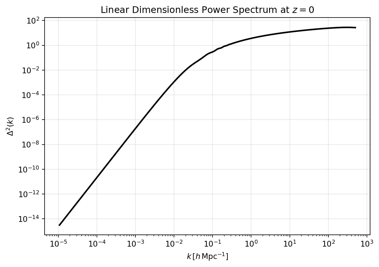
Next, we compute \(\sigma(M)\) by integrating the power spectrum with a top-hat filter. We’ll set up a grid of masses from \(10^{12}\) to \(10^{16}\,M_\odot/h\), compute the corresponding radii, and then perform the integration for each mass.
We’ll use the spherical top-hat window function in Fourier space: \[ W(kR) = \frac{3}{(kR)^3} \left[\sin(kR) - kR \cos(kR)\right] \]
For the integration, we’ll use the trapezoidal rule from numpy on a uniform grid in \(\ln k\), integrating the equivalent form \[
\sigma^2(R) = \int \Delta^2(k)\,W^2(kR)\,\mathrm{d}\ln k.
\] And then, we’ll interpolate \(\ln \sigma\) as a function of \(\ln M\) for later use.
As a test, we’ll also compute \(\sigma(R=8\,\mathrm{Mpc}/h)\), i.e. \(\sigma_8\). The expected value for the Quijote cosmology is 0.834.
from scipy.interpolate import CubicSpline

def top_hat_window(kR):
    """Spherical top-hat window function in Fourier space."""
    kR = np.asarray(kR)
    window = np.empty_like(kR, dtype=float)
    small = np.abs(kR) < 1e-3
    x = kR[small]
    window[small] = 1.0 - x**2 / 10.0 + x**4 / 280.0
    xs = kR[~small]
    window[~small] = 3.0 * (np.sin(xs) - xs * np.cos(xs)) / (xs**3)
    return window

# Constants
rho_m0 = 2.775e11 * 0.3175  # Mean matter density at z=0 in M_sun/h / (Mpc/h)^3

# Mass and radius grids
M_grid = np.logspace(12, 16, 200)  # M_sun/h
R_grid = (3.0 * M_grid / (4.0 * np.pi * rho_m0)) ** (1.0 / 3.0)  # Mpc/h

# Build a uniform ln k grid and interpolate Delta^2(k) onto it
lnk_data = np.log(k_linear)
ln_delta2_data = np.log(delta2_linear)

lnk_uniform = np.linspace(lnk_data.min(), lnk_data.max(), 4096)
delta2_uniform = np.exp(np.interp(lnk_uniform, lnk_data, ln_delta2_data))
k_uniform = np.exp(lnk_uniform)

# Compute sigma(M)
sigma2_grid = np.empty_like(M_grid)

for i, radius in enumerate(R_grid):
    window = top_hat_window(k_uniform * radius)
    integrand = delta2_uniform * (window**2)
    sigma2_grid[i] = np.trapezoid(integrand, lnk_uniform)

sigma_grid = np.sqrt(np.maximum(sigma2_grid, 0.0))

# Interpolate ln sigma as a function of ln M for later Press-Schechter use
ln_sigma_spline = CubicSpline(
    np.log(M_grid),
    np.log(sigma_grid),
    extrapolate=True,
)

# Plot sigma(M)
plt.figure(figsize=(7, 5))
plt.plot(M_grid, sigma_grid, color='k', lw=2)
plt.xscale('log')
plt.yscale('log')
plt.xlabel(r"$M\,[M_\odot/h]$")
plt.ylabel(r"$\sigma(M)$")
plt.title(r"Linear Variance $\sigma(M)$ at $z=0$")
plt.grid(alpha=0.3)
plt.tight_layout()
plt.show()

# Test value: sigma(R=8 Mpc/h), i.e. sigma_8
R8 = 8.0  # Mpc/h
W8 = top_hat_window(k_uniform * R8)
integrand8 = delta2_uniform * (W8**2)
sigma8 = np.sqrt(np.trapezoid(integrand8, lnk_uniform))
print(f"sigma(R=8 Mpc/h) = {sigma8:.4f}")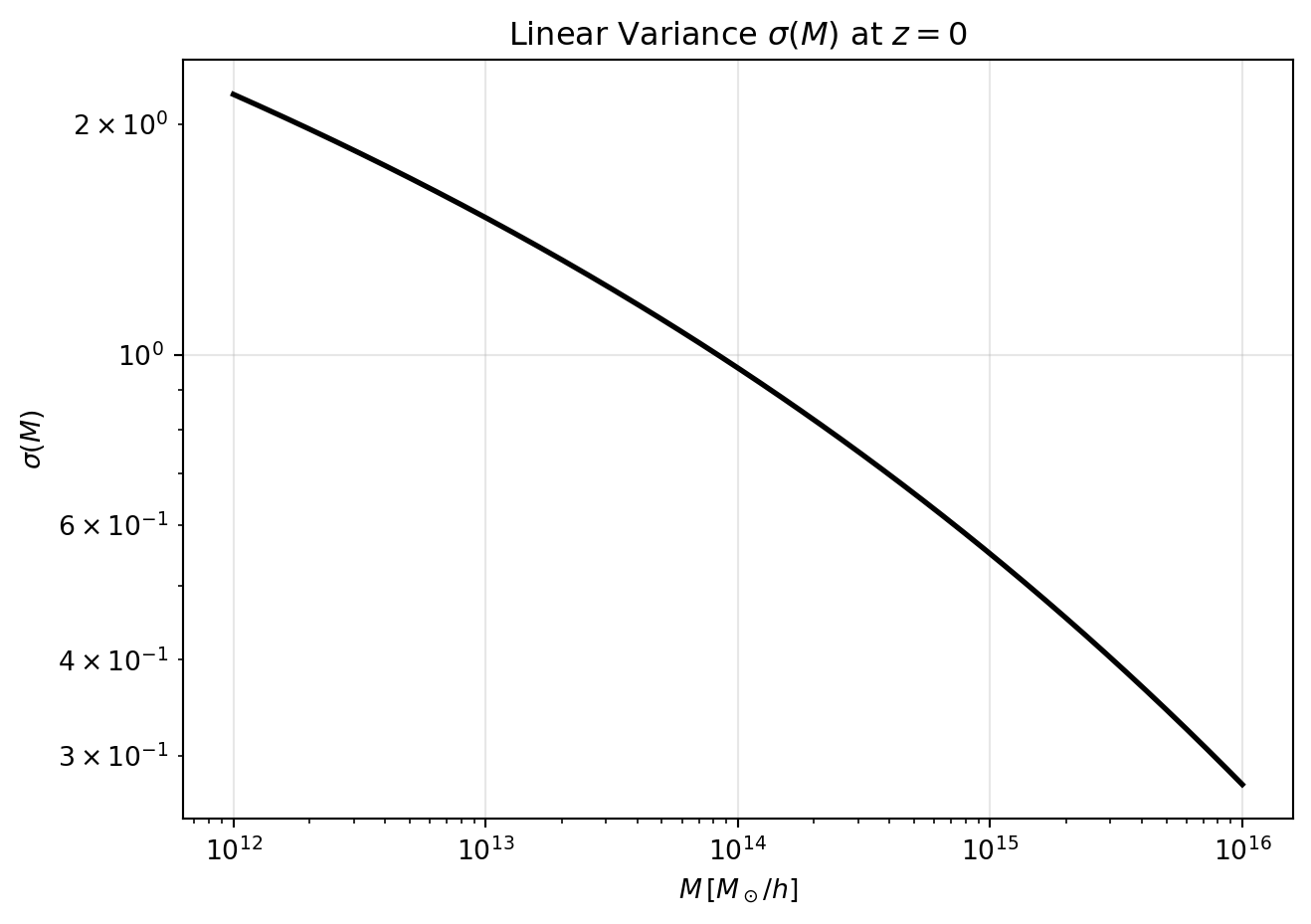
sigma(R=8 Mpc/h) = 0.8340We can now compute the mass function using the Press-Schechter formula and then compare with the Quijote results.
delta_c = 1.686

# Evaluate sigma and its logarithmic derivative on a finer mass grid for theory
M_theory = 10**np.linspace(mass_bins[0], mass_bins[-1], 400)
lnM_theory = np.log(M_theory)
ln_sigma_theory = ln_sigma_spline(lnM_theory)
sigma_theory = np.exp(ln_sigma_theory)

# d ln sigma / d ln M directly from spline derivative
dlnsigma_dlnM_theory = ln_sigma_spline.derivative()(lnM_theory)

# Press-Schechter dn/dlnM
nu_theory = delta_c / sigma_theory
ps_mass_function = (
    np.sqrt(2.0 / np.pi)
    * (rho_m0 / M_theory)
    * nu_theory
    * np.exp(-0.5 * nu_theory**2)
    * np.abs(dlnsigma_dlnM_theory)
)

# Single comparison plot
plt.figure(figsize=(7, 5))
for dndlnM in mass_functions:
    mask = dndlnM > 0
    plt.plot(mass_centers[mask], dndlnM[mask], color='0.75', lw=1.0)

mask_quijote = mean_mass_function > 0
mask_ps = ps_mass_function > 0
plt.plot(
    mass_centers[mask_quijote],
    mean_mass_function[mask_quijote],
    color='k',
    lw=2.5,
    label='Quijote mean',
)
plt.plot(
    M_theory[mask_ps],
    ps_mass_function[mask_ps],
    color='tab:blue',
    lw=2.0,
    ls='--',
    label='Press-Schechter',
)
plt.xscale('log')
plt.yscale('log')
plt.xlabel(r"$M\,[M_\odot/h]$")
plt.ylabel(r"$\mathrm{d}n/\mathrm{d}\ln M\;[(\mathrm{Mpc}/h)^{-3}]$")
plt.title("Halo Mass Function at $z=0$")
plt.grid(alpha=0.3)
plt.legend()
plt.tight_layout()
plt.show()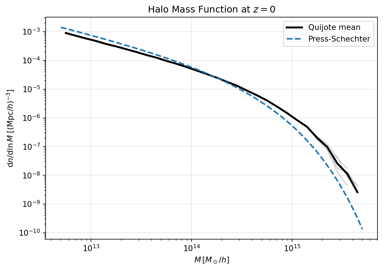
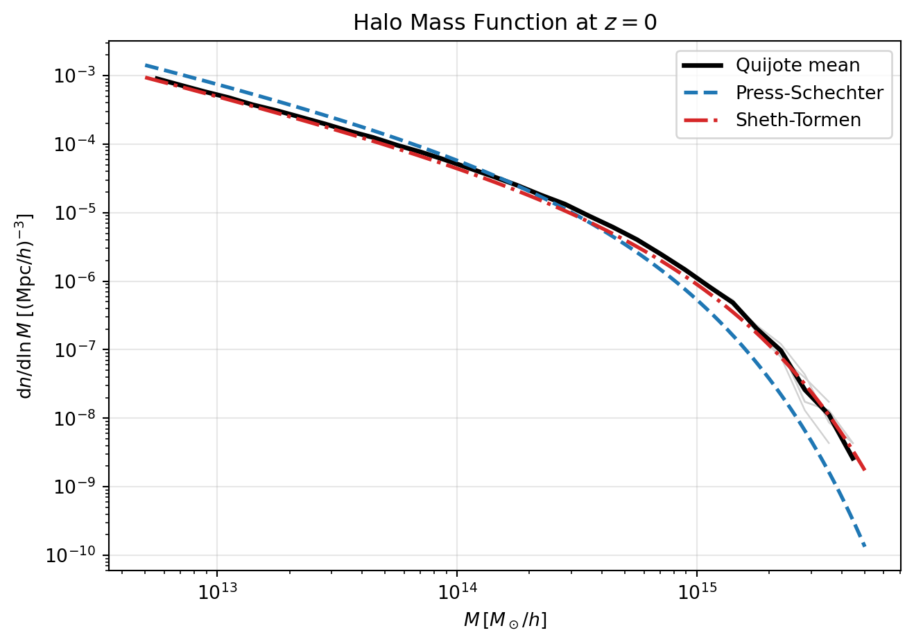
The Press-Schechter multiplicity function is \[ f_{\mathrm{PS}}(\nu) = \sqrt{\frac{2}{\pi}}\,\nu\,e^{-\nu^2/2}. \]
The Sheth-Tormen form modifies this to better match simulation-based halo abundances: \[ f_{\mathrm{ST}}(\nu) = A\,\sqrt{\frac{2a}{\pi}}\,\nu\left[1+(a\nu^2)^{-p}\right]e^{-a\nu^2/2}, \] with typical parameters \(A=0.3222\), \(a=0.707\), and \(p=0.3\).
Using either multiplicity function, \[ \frac{\mathrm{d}n}{\mathrm{d}\ln M} = \frac{\bar{\rho}}{M}f(\nu)\left|\frac{\mathrm{d}\ln\sigma}{\mathrm{d}\ln M}\right|. \]
# Sheth-Tormen multiplicity parameters
A_st = 0.3222
a_st = 0.707
p_st = 0.3

# Sheth-Tormen dn/dlnM on the same theory mass grid
f_st = (
    A_st
    * np.sqrt(2.0 * a_st / np.pi)
    * nu_theory
    * (1.0 + (a_st * nu_theory**2) ** (-p_st))
    * np.exp(-0.5 * a_st * nu_theory**2)
)
st_mass_function = (rho_m0 / M_theory) * f_st * np.abs(dlnsigma_dlnM_theory)

# Plot Quijote + Press-Schechter + Sheth-Tormen
plt.figure(figsize=(7, 5))
for dndlnM in mass_functions:
    mask = dndlnM > 0
    plt.plot(mass_centers[mask], dndlnM[mask], color='0.82', lw=0.9)

mask_quijote = mean_mass_function > 0
mask_ps = ps_mass_function > 0
mask_st = st_mass_function > 0

plt.plot(
    mass_centers[mask_quijote],
    mean_mass_function[mask_quijote],
    color='k',
    lw=2.5,
    label='Quijote mean',
)
plt.plot(
    M_theory[mask_ps],
    ps_mass_function[mask_ps],
    color='tab:blue',
    lw=2.0,
    ls='--',
    label='Press-Schechter',
)
plt.plot(
    M_theory[mask_st],
    st_mass_function[mask_st],
    color='tab:red',
    lw=2.0,
    ls='-.',
    label='Sheth-Tormen',
)

plt.xscale('log')
plt.yscale('log')
plt.xlabel(r"$M\,[M_\odot/h]$")
plt.ylabel(r"$\mathrm{d}n/\mathrm{d}\ln M\;[(\mathrm{Mpc}/h)^{-3}]$")
plt.title("Halo Mass Function at $z=0$")
plt.grid(alpha=0.3)
plt.legend()
plt.tight_layout()
plt.show()