15 Introduction to Linear Perturbations
We now turn to inhomogeneities in the Universe and how these evolve with time. Our treatment here will be limited to the Newtonian regime - so considering velocities \(\ll c\) and length scales much smaller than the horizon. It turns out that these scales are important when considering much of the scales of current galaxy surveys and so, making this approximation is both justified and relevant.
We will consider both baryons and dark matter here, and there will be places where we will distinguish between the two.
The treatment here follows Chap. 5 in Baumann closely.
15.1 Motivation
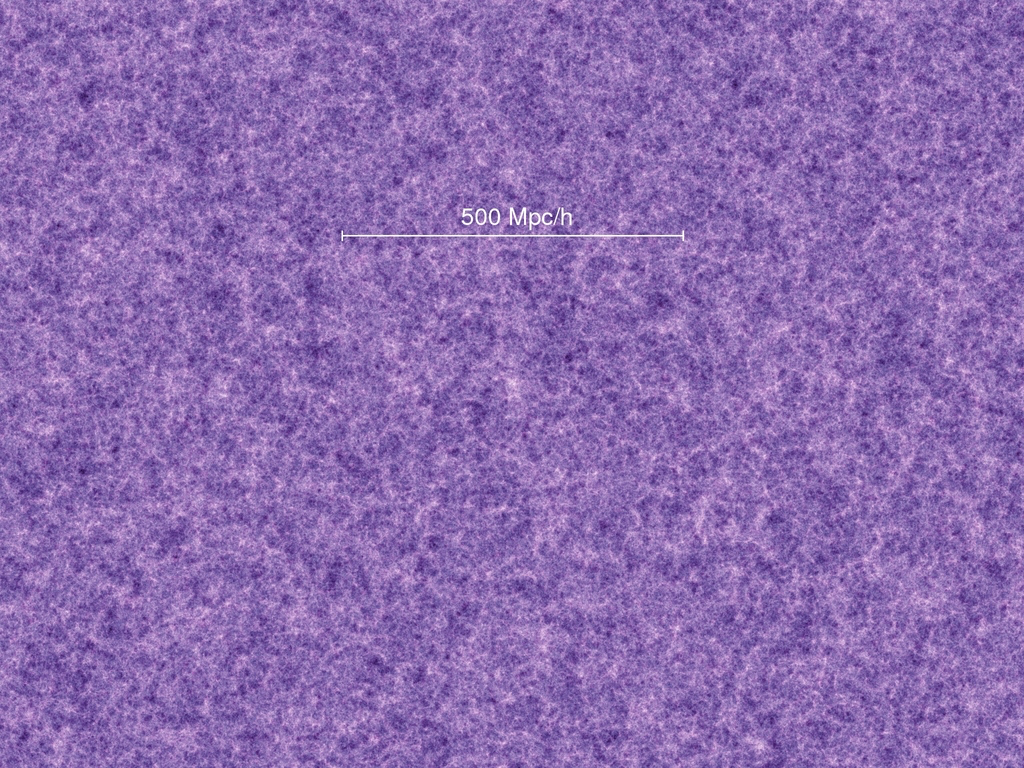
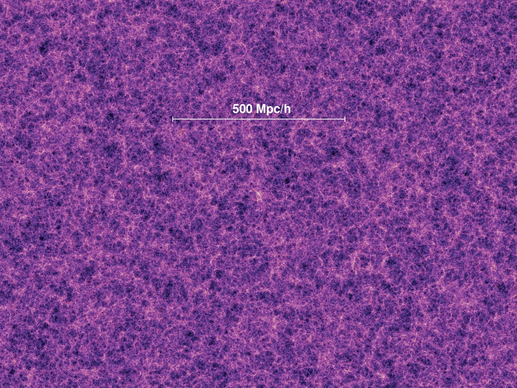
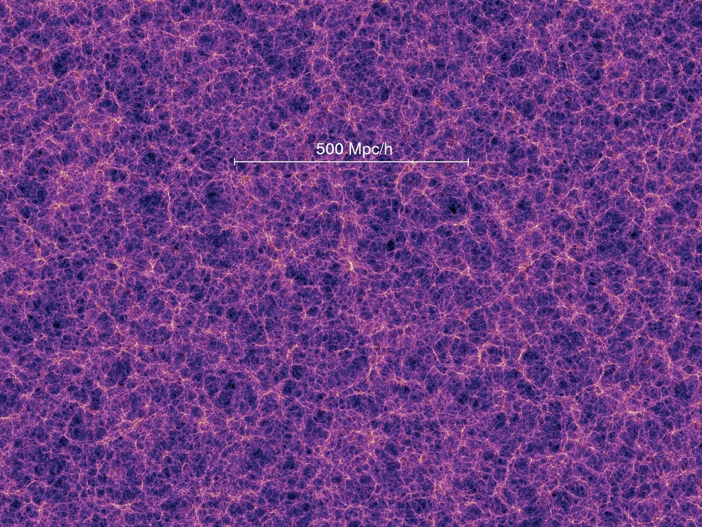
To motivate our discussion, consider the following sequence of snapshots of the dark matter distribution from the Millennium simulation, showing the evolution of the cosmic web as a function of time. As we see, structures grow with time from small perturbations in the early Universe through gravitation and form the cosmic web that we see today.
z=18.3
z=5.7
z=1.4
z=0 (today!)
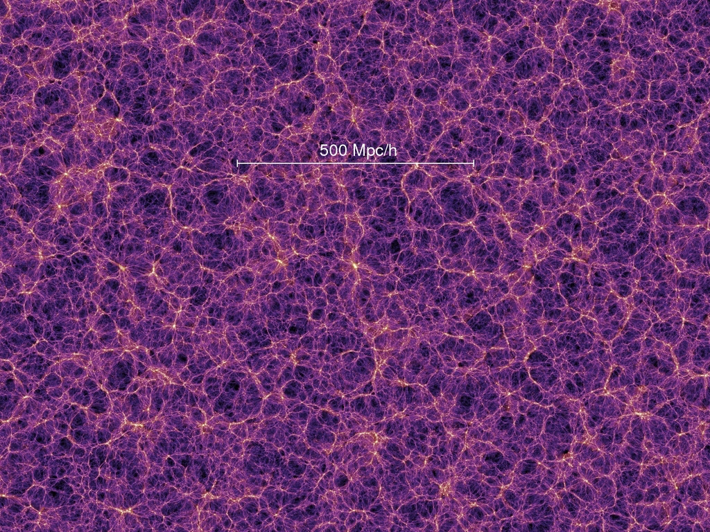
As we go forward in time, we see that the fluctuations grow from small perturbations on all scales to large, nonlinear fluctuations. However, even today, if we average over a large enough volume, we will find that the perturbations can be made small (this is a consequence of our assumption of the homogeneity of the Universe on the largest scales), and linear perturbation theory is a good description. This will be our immediate focus.
Just to summarize the regime of linear perturbation theory : early times and/or large scales.
15.2 Fluid Dynamics
We will treat the matter as a fluid with a mass density \(\rho\), a pressure \(P \ll \rho\) and a velocity \(\mathbf{u} \ll c\). We’ll start by ignoring gravity and the expansion of the Universe, adding these in turn.
The two primary equations governing this fluid are the continuity equation and the Euler equation. The continuity equation \[ \frac{\partial \rho}{\partial t} + \nabla \cdot (\rho \mathbf{u}) = 0 \] captures mass conservation - the change in mass in a given volume per unit time is determined by the flow of material in/out of the volume. The Euler equation follows from momentum conservation and is written as \[ \rho \frac{D \mathbf{u}}{Dt} = \rho \left( \frac{\partial }{\partial t} + \mathbf{u} \cdot \nabla \right) \mathbf{u} = -\nabla P \] Note the appearance of the material or convective derivative \(D/Dt\) to track the a fluid element as it flows. Finally, we close this system with an equation of state to relate pressure to density - we assume a simple form \[ P = P(\rho) \]
An initial solution to this is a static fluid with a uniform density \(\bar{\rho}\), a uniform pressure \(\bar{P}\) and zero fluid velocity \(\mathbf{u}=0\). Let us consider perturbations around this solution \[ \begin{aligned} \rho = \bar{\rho} + \delta \rho \\ P = \bar{P} + \delta P \end{aligned} \] where the perturbations are assumed to functions of space and time. Plugging first into the continuity equation, we find \[ \frac{\partial \delta \rho}{\partial t} = - \bar{\rho} \nabla \cdot \mathbf{u} \] where we are working to linear order and so ignore products of perturbations (note that \(\mathbf{u}\) is a perturbation about the static solution). Similarly, the Euler equation simplifies to \[ \bar{\rho} \frac{\partial \mathbf{u}}{\partial t} = -\nabla \delta P \] We can combine these two equations to get \[ \frac{\partial^{2} \delta \rho}{\partial t^{2}} - \nabla^2 \delta P = 0 \] Finally, we can use the equation of state to eliminate \(\delta P\): \[ \delta P = \frac{\partial P}{\partial \rho} \delta \rho = c_{s}^{2} \delta \rho \] where \(c_{s}\) is the speed of sound in the fluid. This gives us \[ \frac{\partial^{2} \delta \rho}{\partial t^{2}} - c_{s}^{2} \nabla^2 \delta \rho = 0 \]
This is nothing but the wave equation. We can solve this using Fourier transforms : \[ \delta \rho(\mathbf{x}, t) = \int \frac{d^{3} k}{(2\pi)^{3}} e^{ i \mathbf{k} \cdot \mathbf{x} } \delta \rho(\mathbf{k}, t) \] where we explicitly re-introduce the space and time dependencies to show the Fourier transform. The Laplacian \(\nabla^2\) operator pulls down two factors of \(i \mathbf{k}\) and we find \[ \int \frac{d^{3}k}{(2\pi)^{3}} \left[ \frac{\partial^{2} \delta \rho(\mathbf{k},t)}{\partial t^{2}} + c_{s}^{2} k^{2} \rho(\mathbf{k},t) = 0 \right] \] This is nothing by a simple harmonic oscillator for each individual \(\mathbf{k}\) mode, and so the solutions are \[ \delta \rho(\mathbf{k}, t) = A_{\mathbf{k}} e^{ -i \omega_{k} t } + B_{\mathbf{k}} e^{ i \omega_{k} t } \] where \(\omega_{k} = c_{s} k\). Putting this back, we see that \[ \delta \rho(\mathbf{x},t) = \int \frac{d^{3}k}{(2\pi)^{3}} \left[ A_{\mathbf{k}} e^{ -i (\omega_{k}t - \mathbf{k} \cdot \mathbf{x}) } + B_{\mathbf{k}} e^{ i (\omega_{k} t + \mathbf{k} \cdot \mathbf{x}) }\right] \] It is convenient to rewrite this as \[ \delta \rho(\mathbf{x},t) = \int \frac{d^{3}k}{(2\pi)^{3}} \left[ A_{\mathbf{k}} e^{ -i (\omega_{k}t - \mathbf{k} \cdot \mathbf{x}) } + B_{-\mathbf{k}} e^{ i (\omega_{k} t - \mathbf{k} \cdot \mathbf{x}) }\right] \] Furthermore, if we require \(\delta \rho\) to be real, we require \(B_{-\mathbf{k}} = A^{*}_{\mathbf{k}}\) to get \[ \delta \rho(\mathbf{x},t) = \int \frac{d^{3}k}{(2\pi)^{3}} \left[ A_{\mathbf{k}} e^{ -i (\omega_{k}t - \mathbf{k} \cdot \mathbf{x}) } + A_{\mathbf{k}}^* e^{ i (\omega_{k} t - \mathbf{k} \cdot \mathbf{x}) }\right] \] which we recognize as the sum of sine and cosine waves.
This Fourier technique will form the basis of many of our following solutions, and we will often just consider the evolution of a each Fourier mode individually.
15.3 Adding Gravity
The gravitational potential \(\Phi\) modifies the Euler equation \[ \rho \left( \frac{\partial }{\partial t} + \mathbf{u} \cdot \nabla \right) \mathbf{u} = -\nabla P - \rho \nabla \Phi \] and introduces the Poisson equation to relate density to the potential \[ \nabla^2 \Phi = 4 \pi G \rho \]
As before, we consider our uniform background solution, but we hit a snag with the Poisson equation since \[ \nabla^2 \bar{\Phi} = 0 \neq 4 \pi G \bar{\rho} \] Let us just ignore this for now (it will get fixed when we introduce expansion) and just introduce a perturbation to the gravitational potential \[ \Phi = \bar{\Phi} + \delta \Phi \] As before, we can linearize to get \[ \begin{aligned} \frac{\partial \delta \rho}{\partial t} = - \bar{\rho} \nabla \cdot \mathbf{u} \\ \bar{\rho} \frac{\partial \mathbf{u}}{\partial t} = -\nabla \delta P - \bar{\rho} \nabla \delta \Phi\\ \nabla^2 \delta \Phi = 4\pi G \delta \rho \\ \delta P = c_{s}^{2} \delta \rho \end{aligned} \] We can combine these the same way to get a single equation \[ \left( \frac{\partial^{2}}{\partial t^{2}} - c_{s}^{2} \nabla^2 - 4\pi G \bar{\rho}\right) \delta \rho = 0 \] or in Fourier space \[ \left( \frac{\partial^{2}}{\partial t^{2}} + c_{s}^{2} k^2 - 4\pi G \bar{\rho}\right) \delta \rho(\mathbf{k},t) = 0 \] We notice there is a critical wavenumber \(k_{J}\) at which the frequency of oscillations is zero. This scale is known as the Jeans scale. At wavenumbers \(k > k_{J}\), the equation behaves like a simple harmonic oscillator, while below this scale, the equation exponentially grows. Recalling that increasing wavenumbers correspond to decreasing physical scales, the above is just the statement that on small scales, pressure fluctuations dominate and you get sound waves, while on large scales, we get gravity dominating.
The Jeans scale is defined as \[ k_{J}^{2} = \frac{4\pi G \bar{\rho}}{c_{s}^{2}} \] For \(k \ll k_{J}\), we have \[ \left( \frac{\partial^{2}}{\partial t^{2}} - 4\pi G \bar{\rho}\right) \delta \rho(\mathbf{k},t) = 0 \] whose solutions are \[ \delta \rho \sim e^{ \pm t/\tau } \] where \(\tau = 1/\sqrt{ 4\pi G \bar{\rho} }\). This is also known as the Jean’s instability.