Code
# Initial imports
import numpy as np
import matplotlib.pyplot as pltAs we mentioned earlier, one is often forced to numerically solve for quantities in a multi-component Universe. This notebook demonstrates this for a few illustrative cases.
A few notes about the notebooks here. These are meant to be self-contained and do not depend on additional files. As a result, certain function definitions might get repeated throughout.
Additionally, these are not meant to be robust software, but rather exploratory code, so in cases, we may use global variables, or hard-code in particular choices.
Finally, we will try to keep the requirements for these notebooks to the minimum. Hopefully, running these on eg. Google Colab would be straightforward.
# Initial imports
import numpy as np
import matplotlib.pyplot as pltWe’ll start by defining a fiducial cosmology that we will use in many of the examples below. As an implementation detail, we’ll store the parameters in a dictionary, and will specify the parameters at the present epoch. We’ll also specify some convenient constants.
We’ll work assuming \(H_0\) = 100h km/s/Mpc, when necessary, but otherwise will just work in \(c/H_0\) units for distances and \(1/H_0\) units for time.
fiducial = {
    'Omega_m': 0.3,       # Matter density parameter
    'Omega_r': 0.0,       # Radiation density parameter
    'Omega_lambda': 0.7,  # Dark energy density parameter
}

# Constants
cbyH0 = 2997.92  # c / H0 in Mpc for H0 = 100h km/s/Mpc
invH0_Gyr = (3.26156e6 * 2997.92)/1e9 # 1/H0 in Gyr for H0 = 100h km/s/Mpc
# For the above - 3.26156e6 is the number of light years in a Mpc,
# and 2997.92 is c/H0 in Mpc, dividing by 1e9 converts years to GyrHere we define a few helper functions that will be useful below.
In order to account for curvature, we need to compute the radius of curvature today, which is given by: \[ R_c = \frac{c/H_0}{\sqrt{|\Omega_k|}} \] where \(\Omega_k = 1 - \Omega_m - \Omega_r - \Omega_\Lambda\). Note that this follows from the Friedmann equation \[ 1 - \Omega_0 = -\frac{c^2 k}{R_0^2 H_0^2} \] and then working in units of \(c/H_0\) for distances.
While this diverges for a flat Universe, we don’t actually ever need to compute it in that case.
def EHubble(cosmo, z):
    """Dimensionless Hubble parameter E(z) = H(z)/H0."""
    Om = cosmo['Omega_m']
    Or = cosmo['Omega_r']
    Ol = cosmo['Omega_lambda']
    Ok = 1.0 - Om - Or - Ol
    return np.sqrt(Om * (1 + z)**3 + Or * (1 + z)**4 + Ol + Ok * (1 + z)**2)

def Sk(cosmo, chi):
    """Comoving angular diameter distance function S_k(chi).

    chi is the comoving radial distance in c/H0 units.
    """
    Ok = 1.0 - cosmo['Omega_m'] - cosmo['Omega_r'] - cosmo['Omega_lambda']
    if Ok > 0:
        sqrtOk = np.sqrt(Ok)
        return (1.0 / sqrtOk) * np.sinh(sqrtOk * chi)
    elif Ok < 0:
        sqrtAbsOk = np.sqrt(-Ok)
        return (1.0 / sqrtAbsOk) * np.sin(sqrtAbsOk * chi)
    else:
return chiWe can now calculate the cosmological distances by numerically integrating \[
\chi(z) = \int_0^z \frac{dz'}{E(z')}
\] For simplicity, we just use the trapezoidal rule here and the corresponding numpy function.
We could use more sophisticated integration methods, and when plotting, we could just accumulate the integral as we go along to avoid repeated calculations. We leave these and other improvements as exercises to the reader.
def comoving_radial_distance(cosmo, z, dz=1e-3):
    """Comoving radial distance chi(z) in c/H0 units."""
    z_vals = np.arange(0, z + dz/2.0, dz)
    E_vals = EHubble(cosmo, z_vals)
    chi = np.trapezoid(1.0 / E_vals, z_vals)
    return chi
Now let’s plot \(d_M = S_k(\chi)\) for our fiducial cosmology, but also for some additional choices :
This figure is comparable to Fig. 3.2 in Huterer.
# Define cosmologies to compare
cosmo_list = [
    {'name': 'Pure Lambda', 'params': {'Omega_m': 0.0, 'Omega_r': 0.0, 'Omega_lambda': 1.0}},
    {'name': 'Einstein-de Sitter', 'params': {'Omega_m': 1.0, 'Omega_r': 0.0, 'Omega_lambda': 0.0}},
    {'name': 'Open LCDM', 'params': {'Omega_m': 0.2, 'Omega_r': 0.0, 'Omega_lambda': 0.3}},
    {'name': 'Fiducial', 'params': fiducial},
    {'name': 'Closed LCDM', 'params': {'Omega_m': 0.4, 'Omega_r': 0.0, 'Omega_lambda': 0.8}}
]

# Redshift range
z_vals = np.linspace(0, 2, 50)
fig, ax = plt.subplots(figsize=(8, 6))
for cosmo_entry in cosmo_list:
    cosmo = cosmo_entry['params']
    name = cosmo_entry['name']
    chi_vals = [comoving_radial_distance(cosmo, z) for z in z_vals]
    dM_vals = Sk(cosmo, np.array(chi_vals))
    ax.plot(z_vals, np.array(dM_vals), label=name)
ax.set_xlabel('Redshift z', fontsize=12)
ax.set_ylabel('Comoving $d_M$ [c/H0]', fontsize=12)
ax.set_title('Comoving Angular Diameter Distance for Different Cosmologies', fontsize=12)
ax.legend()
ax.grid(True, alpha=0.3)
plt.tight_layout()
plt.show()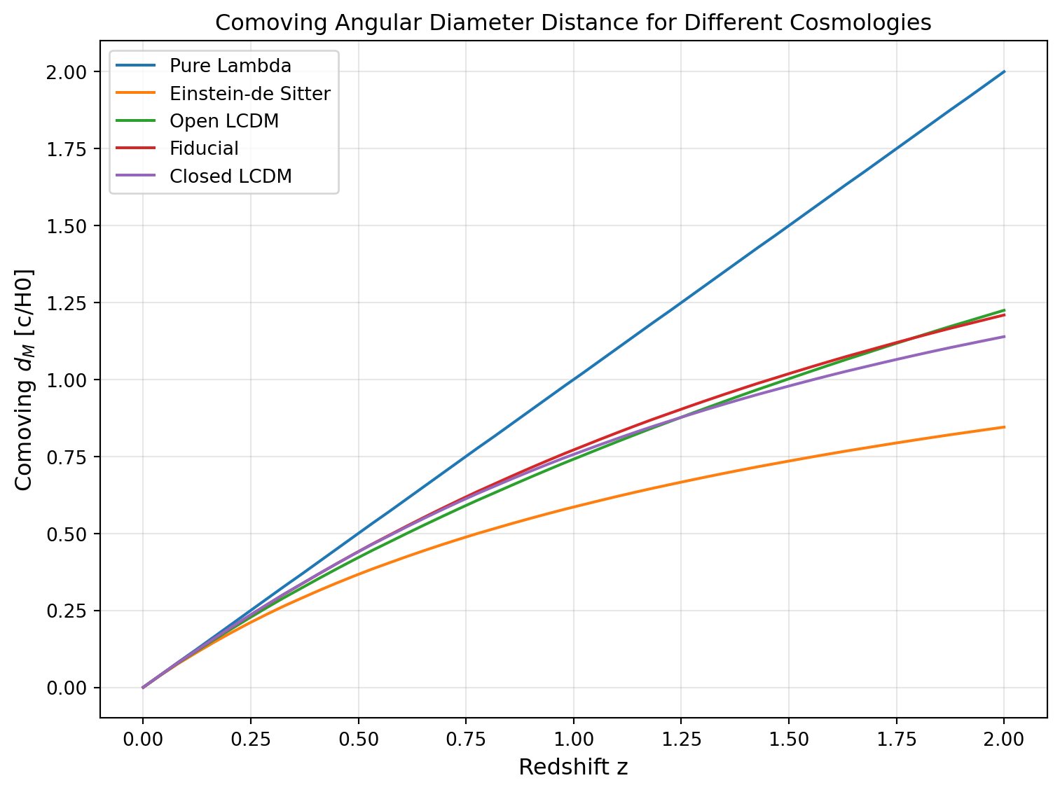
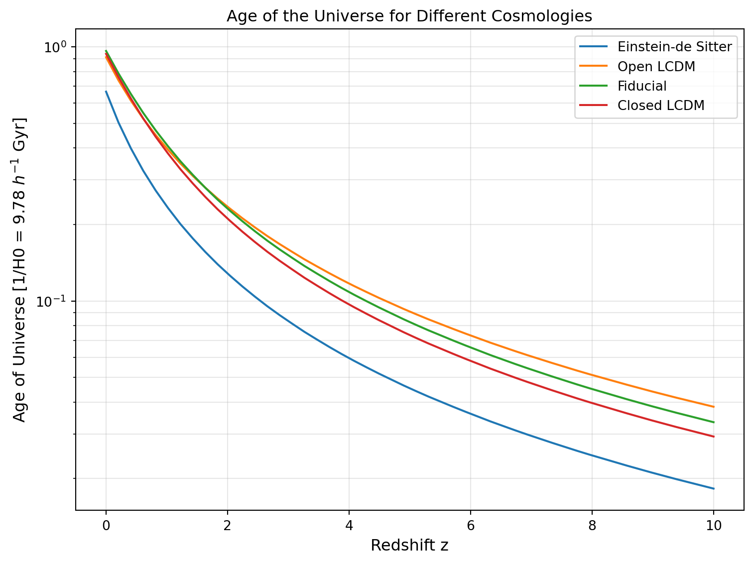
Next, we can compute the age of the Universe at a given redshift by integrating \[ t(a) = \int_{-\infty}^{\log a} \frac{d \log a'}{H(a')} \] where \(H(a) = H_0 E(z)\) as defined above, and \(a = 1/(1+z)\).
We’ll approximate the integral using the trapezoidal rule again, using a large negative number for the lower limit.
Note that we remove the “Lambda” cosmology here, since its age diverges.
def age_of_universe(cosmo, z, dloga=1e-3, loga_min=-20):
    """Age of the Universe at redshift z in 1/H0 units."""
    a = 1.0 / (1.0 + z)
    loga_vals = np.arange(loga_min, np.log(a) + dloga/2.0, dloga)
    a_vals = np.exp(loga_vals)
    z_vals = 1.0 / a_vals - 1.0
    E_vals = EHubble(cosmo, z_vals)
    integrand = 1.0 / (E_vals)
    age = np.trapezoid(integrand, loga_vals)
    return age

# Make a similar plot for ages
# Plot on a log scale in y
z_vals = np.linspace(0, 10, 50)
fig, ax = plt.subplots(figsize=(8, 6))
for cosmo_entry in cosmo_list:
    if cosmo_entry['name'] == 'Pure Lambda':
        continue  # Skip Pure Lambda as its age diverges
    cosmo = cosmo_entry['params']
    name = cosmo_entry['name']
    age_vals = [age_of_universe(cosmo, z) for z in z_vals]
    ax.plot(z_vals, np.array(age_vals), label=name)
ax.set_xlabel('Redshift z', fontsize=12)
ax.set_ylabel('Age of Universe [1/H0 = {:.2f} $h^{{-1}}$ Gyr]'.format(invH0_Gyr), fontsize=12)
ax.set_title('Age of the Universe for Different Cosmologies', fontsize=12)
ax.set_yscale('log')
ax.legend()
ax.grid(True, alpha=0.3, which='both')
plt.tight_layout()
plt.show()