Code
import numpy as np
import matplotlib.pyplot as plt
import pandas as pdAs a worked example, let us take one of the latest supernovae datasets, the Union3 dataset and plot it and then add some simple curves showing different cosmological models. This will build off our previous examples, but we will keep this notebook fully self-contained for pedagogical purposes.
References :
import numpy as np
import matplotlib.pyplot as plt
import pandas as pdWe use pandas to read the data directly from the URL. The data file is whitespace-separated with a comment header line. We only need the zhel (heliocentric redshift) and mb (distance modulus) columns.
# URLs for the Union3 data
data_url = "https://raw.githubusercontent.com/CobayaSampler/sn_data/refs/heads/master/Union3/lcparam_full.txt"
cov_url = "https://raw.githubusercontent.com/CobayaSampler/sn_data/refs/heads/master/Union3/mag_covmat.txt"

# Read the data table
# The header line starts with '# ', so we strip the comment marker
data = pd.read_csv(data_url, sep=r'\s+', comment='#', header=None,
                   names=['name', 'zcmb', 'zhel', 'dz', 'mb', 'dmb', 'x1', 'dx1',
                          'color', 'dcolor', '3rdvar', 'd3rdvar', 'cov_m_s',
                          'cov_m_c', 'cov_s_c', 'set', 'ra', 'dec', 'biascor'])

# Extract the columns we need
zhel = data['zhel'].values  # Heliocentric redshift
mu = data['mb'].values      # Distance modulus

print(f"Loaded {len(zhel)} supernovae")
print(f"Redshift range: {zhel.min():.3f} to {zhel.max():.3f}")
Loaded 22 supernovae
Redshift range: 0.050 to 2.262The covariance matrix file contains the full covariance matrix for the distance modulus measurements. We’ll extract the diagonal elements to get the variance (and hence the error) for each supernova.
# Read the covariance matrix
# First line is the dimension, then the flattened matrix
cov_data = np.loadtxt(cov_url)
n = int(cov_data[0])  # First element is the dimension
cov_matrix = cov_data[1:].reshape(n, n)

# Extract errors from the diagonal
mu_err = np.sqrt(np.diag(cov_matrix))

print(f"Covariance matrix shape: {cov_matrix.shape}")
print(f"Typical distance modulus error: {np.median(mu_err):.3f}")
Covariance matrix shape: (22, 22)
Typical distance modulus error: 0.095We need functions to compute the luminosity distance for different cosmological models. We follow previous notebooks here.
One additional difference is the the SNe analyses plot the distance modulus \[ \mu = m - M = 5 \log_{10} \left( \frac{d_L(z)}{10 \, \text{pc}} \right) \] If we choose to measure distances in units of \(c/H_0\), then the distance modulus can be written as \[ \mu = m - M = 5 \log_{10} \left( d_L(z) \right) + \text{offset} \] where the offset absorbs the unit conversion (approximately 43.16 for \(h \sim 0.7\)) as well as uncertainties in the absolute magnitude of the SNe.
def EHubble(cosmo, z):
    """Dimensionless Hubble parameter E(z) = H(z)/H0."""
    Om = cosmo['Omega_m']
    Ol = cosmo['Omega_lambda']
    Ok = 1.0 - Om - Ol
    return np.sqrt(Om * (1 + z)**3 + Ol + Ok * (1 + z)**2)

def Sk(cosmo, chi):
    """Comoving angular diameter distance function S_k(chi).

    chi is the comoving radial distance in c/H0 units.
    """
    Ok = 1.0 - cosmo['Omega_m'] - cosmo['Omega_lambda']
    if Ok > 0:
        sqrtOk = np.sqrt(Ok)
        return (1.0 / sqrtOk) * np.sinh(sqrtOk * chi)
    elif Ok < 0:
        sqrtAbsOk = np.sqrt(-Ok)
        return (1.0 / sqrtAbsOk) * np.sin(sqrtAbsOk * chi)
    else:
        return chi

def comoving_radial_distance(cosmo, z, dz=1e-3):
    """Comoving radial distance chi(z) in c/H0 units."""
    z_vals = np.arange(0, z + dz/2.0, dz)
    E_vals = EHubble(cosmo, z_vals)
    chi = np.trapezoid(1.0 / E_vals, z_vals)
    return chi

def luminosity_distance(cosmo, z):
    """Luminosity distance d_L(z) in c/H0 units."""
    chi = comoving_radial_distance(cosmo, z)
    dM = Sk(cosmo, chi)
    return (1 + z) * dM

def distance_modulus(cosmo, z, offset):
    """Distance modulus for a given cosmology.

    The distance modulus is μ = 5*log10(d_L/10pc).
    With d_L in c/H0 units, we have μ = 5*log10(d_L) + offset,
    where the offset absorbs the unit conversion (approximately 43.16 for h~0.7)
    as well as uncertainties in the absolute magnitude of the SNe.
    """
    dL = luminosity_distance(cosmo, z)
return offset + 5 * np.log10(dL)We define four cosmological models to compare with the data:
We fit the offset to the fiducial model, then use that same value for the other models to show how they deviate from the data.
This is a much simplified approach. A more complete analysis would fit for the cosmological parameters and the offset simultaneously.
# Define the cosmological models
cosmo_fiducial = {'Omega_m': 0.3, 'Omega_lambda': 0.7}
cosmo_open = {'Omega_m': 0.3, 'Omega_lambda': 0.0}
cosmo_EdS = {'Omega_m': 1.0, 'Omega_lambda': 0.0}
cosmo_dS = {'Omega_m': 0.0, 'Omega_lambda': 1.0}

# Fit offset to the fiducial model (simple least squares)
dL_fiducial = np.array([luminosity_distance(cosmo_fiducial, z) for z in zhel])
offset_fit = np.mean(mu - 5 * np.log10(dL_fiducial))
print(f"Fitted offset = {offset_fit:.3f}")
Fitted offset = 43.012The classic “Hubble diagram” plots apparent magnitude versus redshift, while the SNe versions tend to plot the inferred distance modulus versus redshift.
fig, ax = plt.subplots(figsize=(10, 6))

# Plot the data
ax.errorbar(zhel, mu, yerr=mu_err, fmt='o', markersize=5,
            alpha=0.7, capsize=0, elinewidth=0.5, label='Union3 SNe Ia')

# Plot model curves - extend to maximum redshift in data
z_model = np.linspace(0.01, zhel.max(), 100)

for cosmo, name, ls in [(cosmo_fiducial, r'$\Omega_m=0.3, \Omega_\Lambda=0.7$', '-'),
                         (cosmo_open, r'$\Omega_m=0.3, \Omega_\Lambda=0$', '--'),
                         (cosmo_EdS, r'$\Omega_m=1.0, \Omega_\Lambda=0$', ':'),
                         (cosmo_dS, r'$\Omega_m=0, \Omega_\Lambda=1$', '-.')]:
    mu_model = np.array([distance_modulus(cosmo, z, offset_fit) for z in z_model])
    ax.plot(z_model, mu_model, ls, lw=2, label=name)

ax.set_xlabel('Heliocentric Redshift $z_{hel}$', fontsize=12)
ax.set_ylabel(r'Distance Modulus $\mu$', fontsize=12)
ax.set_title('Union3 Supernovae Ia Hubble Diagram', fontsize=14)

ax.legend()
ax.grid(True, alpha=0.3)
plt.tight_layout()
plt.show()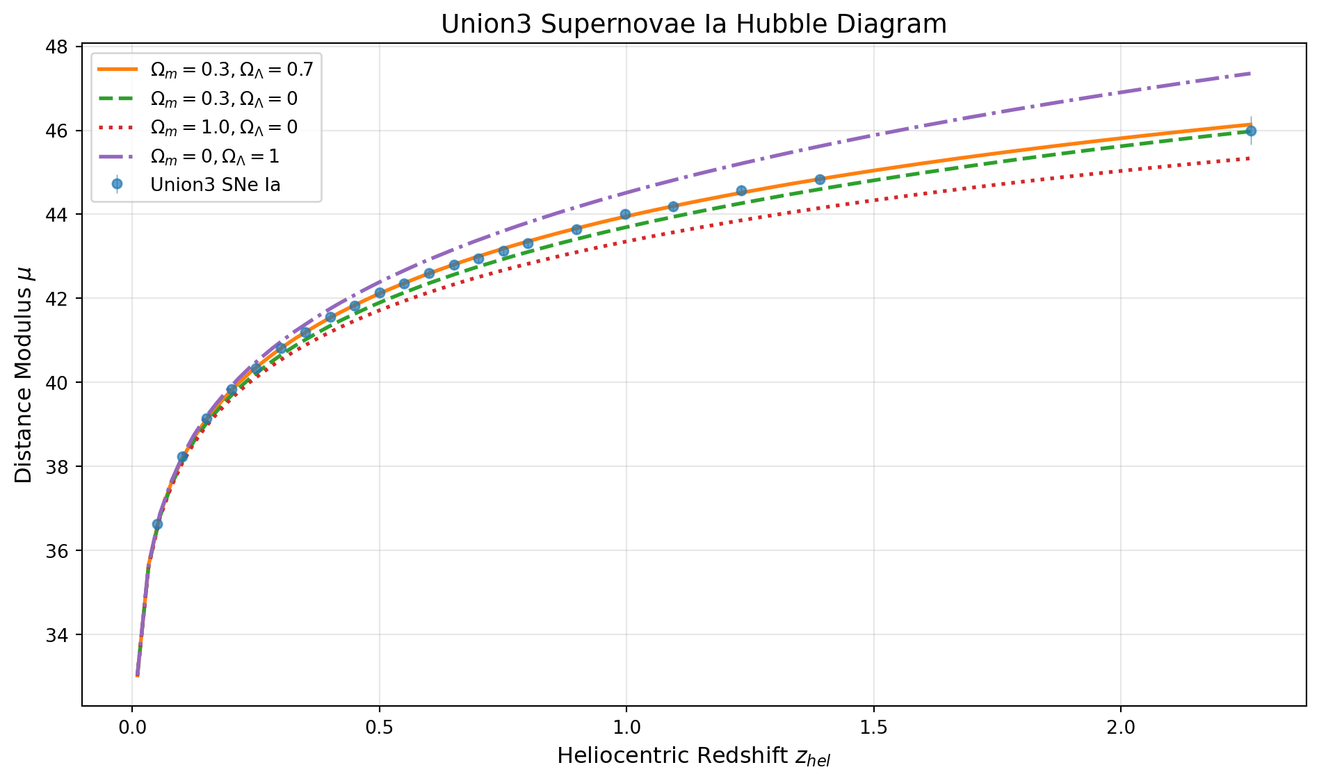
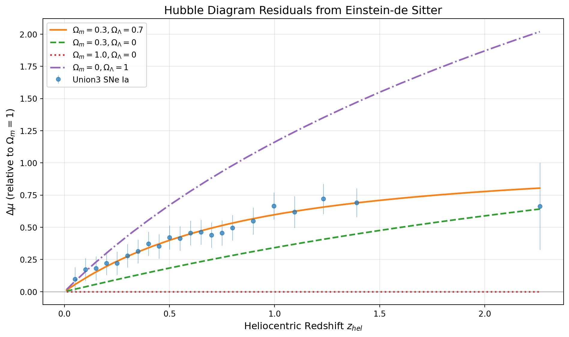
To better see the differences between models, we plot the residuals relative to the Einstein-de Sitter (\(\Omega_m = 1\)) model. This is a common way to visualize the evidence for dark energy.
fig, ax = plt.subplots(figsize=(10, 6))

# Compute EdS prediction for the data points
mu_EdS_data = np.array([distance_modulus(cosmo_EdS, z, offset_fit) for z in zhel])

# Plot data residuals
ax.errorbar(zhel, mu - mu_EdS_data, yerr=mu_err, fmt='o', markersize=5,
            alpha=0.7, capsize=0, elinewidth=0.5, label='Union3 SNe Ia')

# Plot model residuals
mu_EdS_model = np.array([distance_modulus(cosmo_EdS, z, offset_fit) for z in z_model])

for cosmo, name, ls in [(cosmo_fiducial, r'$\Omega_m=0.3, \Omega_\Lambda=0.7$', '-'),
                         (cosmo_open, r'$\Omega_m=0.3, \Omega_\Lambda=0$', '--'),
                         (cosmo_EdS, r'$\Omega_m=1.0, \Omega_\Lambda=0$', ':'),
                         (cosmo_dS, r'$\Omega_m=0, \Omega_\Lambda=1$', '-.')]:
    mu_model = np.array([distance_modulus(cosmo, z, offset_fit) for z in z_model])
    ax.plot(z_model, mu_model - mu_EdS_model, ls, lw=2, label=name)

ax.axhline(0, color='gray', lw=1, alpha=0.5)
ax.set_xlabel('Heliocentric Redshift $z_{hel}$', fontsize=12)
ax.set_ylabel(r'$\Delta \mu$ (relative to $\Omega_m=1$)', fontsize=12)
ax.set_title('Hubble Diagram Residuals from Einstein-de Sitter', fontsize=14)

ax.legend()
ax.grid(True, alpha=0.3)
plt.tight_layout()
plt.show()