9 Numerically Integrating the Friedmann Equation with JAX and Diffrax

This notebook demonstrates numerical solution of cosmological integrals using JAX and Diffrax, reformulating them as ordinary differential equations (ODEs). This approach enables automatic differentiation of cosmological quantities with respect to parameters, which is useful for parameter inference and sensitivity analysis.

We’ll compute the same quantities as in the basic numerical integration notebook but using a modern differentiable programming framework. This allows us to:

Use adaptive ODE solvers (Dormand-Prince 5(4)) with automatic step control
Compute derivatives with respect to cosmological parameters via autodiff
Validate against analytical solutions for single-component universes

A few notes about the notebooks here. These are meant to be self-contained and do not depend on additional files. As a result, certain function definitions might get repeated throughout.

Additionally, these are not meant to be robust software, but rather exploratory code, so in cases, we may use global variables, or hard-code in particular choices.

9.1 Running on Google Colab

To run this notebook on Google Colab, you’ll need to install JAX and Diffrax:

!pip install jax jaxlib diffrax

For more details on JAX installation options, see: https://jax.readthedocs.io/en/latest/installation.html

Code

# Initial imports
import jax
import jax.numpy as jnp
from jax import grad, vmap, jit
import diffrax
import matplotlib.pyplot as plt

9.2 The Fiducial Cosmology

We’ll start by defining a fiducial cosmology that we will use in many of the examples below. As an implementation detail, we’ll store the parameters in a dictionary, and will specify the parameters at the present epoch. We’ll also specify some convenient constants.

We’ll work assuming \(H_0\) = 100h km/s/Mpc, when necessary, but otherwise will just work in \(c/H_0\) units for distances and \(1/H_0\) units for time.

Code

fiducial = {
    'Omega_m': 0.3,       # Matter density parameter
    'Omega_r': 0.0,       # Radiation density parameter
    'Omega_lambda': 0.7,  # Dark energy density parameter
}

# Constants
cbyH0 = 2997.92  # c / H0 in Mpc for H0 = 100h km/s/Mpc
invH0_Gyr = (3.26156e6 * 2997.92)/1e9 # 1/H0 in Gyr for H0 = 100h km/s/Mpc
# For the above - 3.26156e6 is the number of light years in a Mpc,
# and 2997.92 is c/H0 in Mpc, dividing by 1e9 converts years to Gyr

9.3 Useful Functions

Here we define a few helper functions that will be useful below. These are rewritten to use JAX numpy (jnp) instead of regular numpy to enable automatic differentiation.

In order to account for curvature, we need to compute the radius of curvature today, which is given by: \[ R_c = \frac{c/H_0}{\sqrt{|\Omega_k|}} \] where \(\Omega_k = 1 - \Omega_m - \Omega_r - \Omega_\Lambda\). Note that this follows from the Friedmann equation \[ 1 - \Omega_0 = -\frac{c^2 k}{R_0^2 H_0^2} \] and then working in units of \(c/H_0\) for distances.

While this diverges for a flat Universe, we don’t actually ever need to compute it in that case.

Important for JAX: The Sk function uses jnp.where instead of if/elif/else to ensure compatibility with JAX’s tracing and automatic differentiation. JAX requires that control flow be expressed in a way that can be differentiated.

Code

def EHubble(cosmo, z):
    """Dimensionless Hubble parameter E(z) = H(z)/H0."""
    Om = cosmo['Omega_m']
    Or = cosmo['Omega_r']
    Ol = cosmo['Omega_lambda']
    Ok = 1.0 - Om - Or - Ol
    return jnp.sqrt(Om * (1 + z)**3 + Or * (1 + z)**4 + Ol + Ok * (1 + z)**2)

def Sk(cosmo, chi):
    """Comoving angular diameter distance function S_k(chi).

    chi is the comoving radial distance in c/H0 units.
    Uses jnp.where for JAX compatibility instead of if/elif/else.
    """
    Ok = 1.0 - cosmo['Omega_m'] - cosmo['Omega_r'] - cosmo['Omega_lambda']

    # Use a safe sqrt that avoids division by zero for the flat case
    # When |Ok| < 1e-10, we'll return chi anyway, so the dummy value doesn't matter
    sqrtOk_safe = jnp.where(jnp.abs(Ok) > 1e-10, jnp.sqrt(jnp.abs(Ok)), 1.0)

    # Positive curvature (open universe)
    sinh_result = (1.0 / sqrtOk_safe) * jnp.sinh(sqrtOk_safe * chi)

    # Negative curvature (closed universe)
    sin_result = (1.0 / sqrtOk_safe) * jnp.sin(sqrtOk_safe * chi)

    # Select based on Ok value
    result = jnp.where(Ok > 1e-10, sinh_result,
                       jnp.where(Ok < -1e-10, sin_result, chi))
    return result

9.4 Distances with Diffrax

We can calculate the comoving radial distance \(\chi(z)\) by reformulating the integral as an ODE initial value problem:

\[ \frac{d\chi}{dz} = \frac{1}{E(z)}, \quad \chi(0) = 0 \]

This is equivalent to computing: \[ \chi(z) = \int_0^z \frac{dz'}{E(z')} \]

We use Diffrax’s diffeqsolve with the Dopri5 solver (Dormand-Prince 5(4)), which provides adaptive step size control and good accuracy for smooth problems.

Code

def comoving_radial_distance(cosmo, z_final, rtol=1e-8, atol=1e-10):
    """Comoving radial distance chi(z) in c/H0 units using Diffrax ODE solver."""

    def dchi_dz(z, chi, args):
        """ODE: dchi/dz = 1/E(z)"""
        return 1.0 / EHubble(cosmo, z)

    # ODE term
    term = diffrax.ODETerm(dchi_dz)

    # Solver: Dormand-Prince 5(4) with adaptive stepping
    solver = diffrax.Dopri5()

    # Initial condition: chi(z=0) = 0
    t0 = 0.0
    t1 = z_final
    y0 = 0.0

    # Step size controller
    stepsize_controller = diffrax.PIDController(rtol=rtol, atol=atol)

    # Solve the ODE
    sol = diffrax.diffeqsolve(
        term,
        solver,
        t0=t0,
        t1=t1,
        dt0=0.01,  # Initial step size guess
        y0=y0,
        stepsize_controller=stepsize_controller,
    )

    return sol.ys[0]

# Vectorize to handle arrays of redshifts
comoving_radial_distance_vec = vmap(
    lambda z: comoving_radial_distance(fiducial, z),
    in_axes=0
)

Now let’s plot \(d_M = S_k(\chi)\) for our fiducial cosmology, but also for some additional choices :

“Pure Lambda”: \(\Omega_m = 0.0, \Omega_\Lambda = 1.0\)
“Einstein-de Sitter”: \(\Omega_m = 1.0, \Omega_\Lambda = 0.0\)
“Open LCDM”: \(\Omega_m = 0.2, \Omega_\Lambda = 0.3\)
“Fiducial”: our fiducial cosmology defined above.
“Closed LCDM”: \(\Omega_m = 0.4, \Omega_\Lambda = 0.8\)

This figure is comparable to Fig. 3.2 in Huterer.

Code

# Define cosmologies to compare
cosmo_list = [
    {'name': 'Pure Lambda', 'params': {'Omega_m': 0.0, 'Omega_r': 0.0, 'Omega_lambda': 1.0}},
    {'name': 'Einstein-de Sitter', 'params': {'Omega_m': 1.0, 'Omega_r': 0.0, 'Omega_lambda': 0.0}},
    {'name': 'Open LCDM', 'params': {'Omega_m': 0.2, 'Omega_r': 0.0, 'Omega_lambda': 0.3}},
    {'name': 'Fiducial', 'params': fiducial},
    {'name': 'Closed LCDM', 'params': {'Omega_m': 0.4, 'Omega_r': 0.0, 'Omega_lambda': 0.8}}
]

# Redshift range
z_vals = jnp.linspace(0.01, 2, 50)  # Start at 0.01 to avoid z=0
fig, ax = plt.subplots(figsize=(8, 6))
for cosmo_entry in cosmo_list:
    cosmo = cosmo_entry['params']
    name = cosmo_entry['name']
    # Vectorize for this specific cosmology
    chi_func = vmap(lambda z: comoving_radial_distance(cosmo, z), in_axes=0)
    chi_vals = chi_func(z_vals)
    dM_vals = Sk(cosmo, chi_vals)
    ax.plot(z_vals, dM_vals, label=name)
ax.set_xlabel('Redshift z', fontsize=12)
ax.set_ylabel(r'Comoving $d_M$ [c/H0]', fontsize=12)
ax.set_title('Comoving Angular Diameter Distance for Different Cosmologies', fontsize=12)
ax.legend()
ax.grid(True, alpha=0.3)
plt.tight_layout()
plt.show()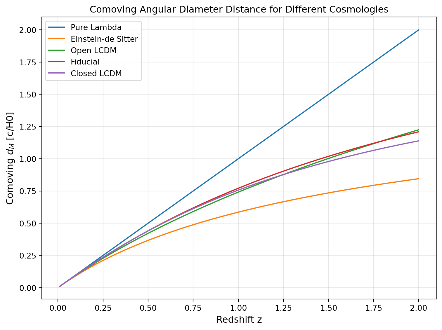

9.5 Ages with Diffrax

Next, we compute the age of the Universe at a given redshift by reformulating the integral as an ODE:

\[ \frac{dt}{d\log a} = \frac{1}{E(z(a))}, \quad t(\log a \to -\infty) \approx 0 \]

where \(a = 1/(1+z)\) is the scale factor and \(E(z) = H(z)/H_0\) as defined above. This is equivalent to: \[ t(a) = \int_{-\infty}^{\log a} \frac{d \log a'}{H(a')} \]

We approximate the integral by starting at a large negative value of \(\log a\) (corresponding to very early times).

Note that we remove the “Pure Lambda” cosmology here, since its age diverges.

Code

def age_of_universe(cosmo, z, loga_min=-20, rtol=1e-8, atol=1e-10):
    """Age of the Universe at redshift z in 1/H0 units using Diffrax ODE solver."""

    a = 1.0 / (1.0 + z)
    loga_final = jnp.log(a)

    def dt_dloga(loga, t, args):
        """ODE: dt/d(log a) = 1/E(z(a))"""
        a_val = jnp.exp(loga)
        z_val = 1.0 / a_val - 1.0
        return 1.0 / EHubble(cosmo, z_val)

    # ODE term
    term = diffrax.ODETerm(dt_dloga)

    # Solver
    solver = diffrax.Dopri5()

    # Initial condition: t(log a -> -infinity) = 0
    t0 = loga_min
    t1 = loga_final
    y0 = 0.0

    # Step size controller
    stepsize_controller = diffrax.PIDController(rtol=rtol, atol=atol)

    # Solve the ODE
    sol = diffrax.diffeqsolve(
        term,
        solver,
        t0=t0,
        t1=t1,
        dt0=0.1,  # Initial step size guess
        y0=y0,
        stepsize_controller=stepsize_controller,
    )

    return sol.ys[0]

# Make a similar plot for ages
# Plot on a log scale in y
z_vals = jnp.linspace(0.01, 10, 50)  # Start at 0.01 to avoid z=0
fig, ax = plt.subplots(figsize=(8, 6))
for cosmo_entry in cosmo_list:
    if cosmo_entry['name'] == 'Pure Lambda':
        continue  # Skip Pure Lambda as its age diverges
    cosmo = cosmo_entry['params']
    name = cosmo_entry['name']
    # Vectorize for this specific cosmology
    age_func = vmap(lambda z: age_of_universe(cosmo, z), in_axes=0)
    age_vals = age_func(z_vals)
    ax.plot(z_vals, age_vals, label=name)
ax.set_xlabel('Redshift z', fontsize=12)
ax.set_ylabel('Age of Universe [1/H0 = {:.2f} $h^{{-1}}$ Gyr]'.format(invH0_Gyr), fontsize=12)
ax.set_title('Age of the Universe for Different Cosmologies', fontsize=12)
ax.set_yscale('log')
ax.legend()
ax.grid(True, alpha=0.3, which='both')
plt.tight_layout()
plt.show()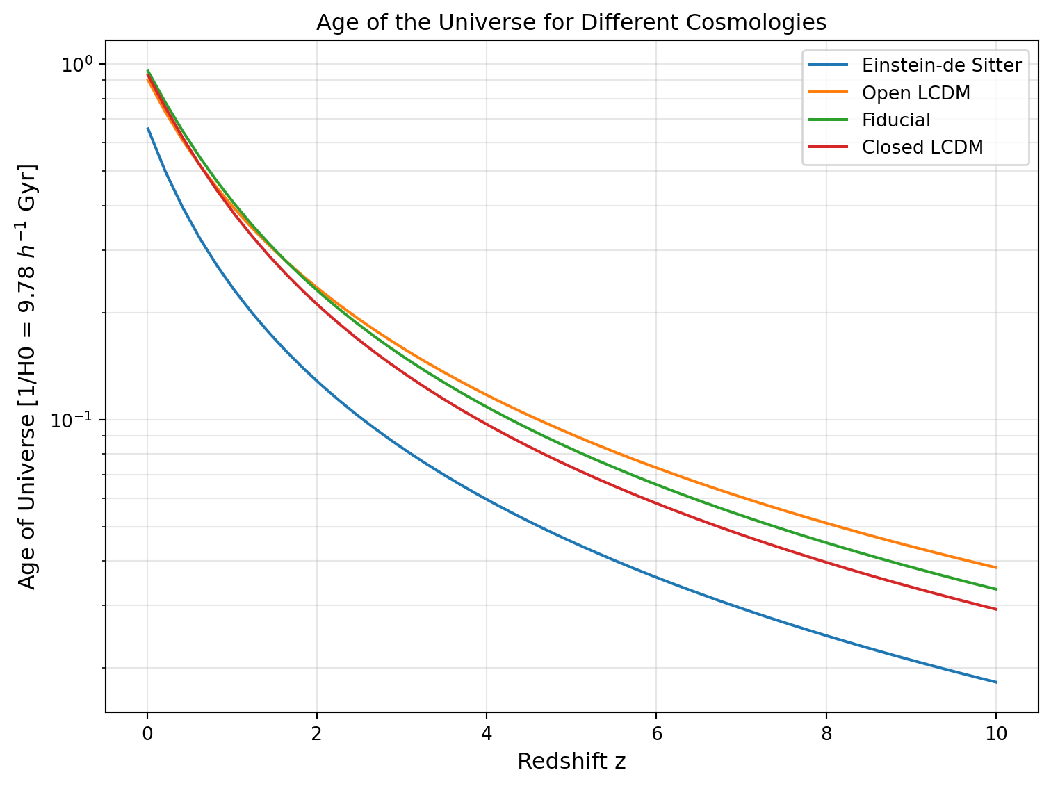

9.6 Automatic Differentiation with JAX

One of the key advantages of using JAX is the ability to compute derivatives of our cosmological quantities with respect to the input parameters using automatic differentiation. This is particularly useful for:

Parameter inference and optimization
Computing Fisher information matrices
Sensitivity analysis

Here we demonstrate computing derivatives of the comoving distance with respect to \(\Omega_m\) and \(\Omega_\lambda\) at a fixed redshift.

For a more complete and production-ready implementation of differentiable cosmology, see the JAX-COSMO library: https://github.com/DifferentiableUniverseInitiative/jax_cosmo

Code

# Define functions to compute derivatives
def chi_wrt_Om(Om, z_eval):
    """Comoving distance as a function of Omega_m."""
    cosmo = {'Omega_m': Om, 'Omega_r': 0.0, 'Omega_lambda': 0.7}
    return comoving_radial_distance(cosmo, z_eval)

def chi_wrt_Ol(Ol, z_eval):
    """Comoving distance as a function of Omega_lambda."""
    cosmo = {'Omega_m': 0.3, 'Omega_r': 0.0, 'Omega_lambda': Ol}
    return comoving_radial_distance(cosmo, z_eval)

# Compute gradients
grad_chi_Om = grad(chi_wrt_Om, argnums=0)
grad_chi_Ol = grad(chi_wrt_Ol, argnums=0)

# Evaluate at sample redshifts for the fiducial cosmology
z_samples = jnp.array([0.5, 1.0, 2.0, 5.0])
Om_fid = 0.3
Ol_fid = 0.7

print("Derivatives of comoving distance chi(z) at fiducial cosmology:")
print("=" * 70)
print(f"{'z':>8} {'chi [c/H0]':>15} {'∂χ/∂Ωm':>15} {'∂χ/∂Ωλ':>15}")
print("-" * 70)

for z in z_samples:
    chi_val = comoving_radial_distance(fiducial, z)
    dchi_dOm = grad_chi_Om(Om_fid, z)
    dchi_dOl = grad_chi_Ol(Ol_fid, z)
    print(f"{z:8.1f} {chi_val:15.6f} {dchi_dOm:15.6f} {dchi_dOl:15.6f}")

Derivatives of comoving distance chi(z) at fiducial cosmology:
======================================================================
       z      chi [c/H0]          ∂χ/∂Ωm          ∂χ/∂Ωλ
----------------------------------------------------------------------
     0.5        0.440984       -0.065449        0.087409
     1.0        0.771427       -0.226072        0.231644
     2.0        1.209471       -0.594746        0.443205
     5.0        1.815509       -1.330786        0.664718

Derivatives vs Redshift

Let’s visualize how these derivatives change as a function of redshift.

Code

# Compute derivatives over a range of redshifts
z_range = jnp.linspace(0.1, 5.0, 50)

# Vectorize gradient computations
grad_Om_vec = vmap(lambda z: grad_chi_Om(Om_fid, z))
grad_Ol_vec = vmap(lambda z: grad_chi_Ol(Ol_fid, z))

dchi_dOm_vals = grad_Om_vec(z_range)
dchi_dOl_vals = grad_Ol_vec(z_range)

# Plot
fig, (ax1, ax2) = plt.subplots(1, 2, figsize=(14, 5))

ax1.plot(z_range, dchi_dOm_vals, 'b-', linewidth=2)
ax1.set_xlabel('Redshift z', fontsize=12)
ax1.set_ylabel(r'$\partial \chi / \partial \Omega_m$ [c/H0]', fontsize=12)
ax1.set_title('Sensitivity to Matter Density', fontsize=12)
ax1.grid(True, alpha=0.3)

ax2.plot(z_range, dchi_dOl_vals, 'r-', linewidth=2)
ax2.set_xlabel('Redshift z', fontsize=12)
ax2.set_ylabel(r'$\partial \chi / \partial \Omega_\Lambda$ [c/H0]', fontsize=12)
ax2.set_title('Sensitivity to Dark Energy Density', fontsize=12)
ax2.grid(True, alpha=0.3)

plt.tight_layout()
plt.show()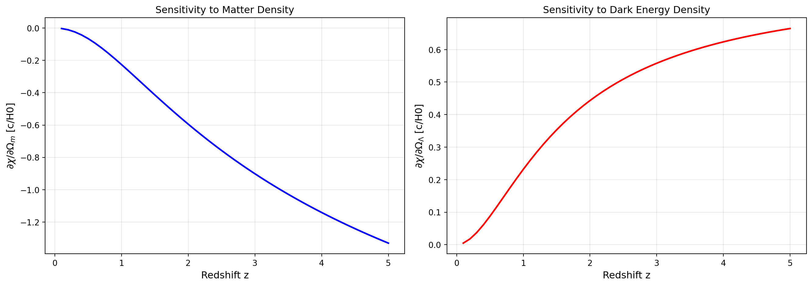

Physical Interpretation

The derivatives tell us how sensitive the comoving distance is to changes in the cosmological parameters:

\(\partial\chi/\partial\Omega_m < 0\): Increasing matter density slows expansion, reducing distances at fixed redshift.
\(\partial\chi/\partial\Omega_\Lambda > 0\): Increasing dark energy density accelerates expansion, increasing distances at fixed redshift.

The magnitude of these derivatives increases with redshift, indicating that high-redshift observations are more sensitive to cosmological parameters. This is why surveys targeting high-redshift objects (like Type Ia supernovae at z > 1 or the CMB at z ~ 1100) are so powerful for constraining cosmology.

These derivatives are the building blocks for computing Fisher information matrices, which predict the parameter constraints achievable from a given dataset. In Bayesian inference, these gradients can be used for efficient gradient-based sampling methods like Hamiltonian Monte Carlo.

9.7 Analytical Validation

To verify our numerical integration, we compare against known analytical solutions for single-component flat universes. For a universe dominated by a single component with equation of state \(w \neq -1\), the comoving distance and age have closed-form expressions.

Matter-Dominated Universe (\(\Omega_m = 1, w = 0\))

For a flat matter-only universe: \[ \chi(z) = \frac{c}{H_0} \frac{2}{1+3w} \left[ 1 - \frac{1}{(1+z)^{(1+3w)/2}} \right] = \frac{2c}{H_0} \left[ 1 - (1+z)^{-1/2} \right] \]

\[ t_0 = \frac{1}{H_0} \frac{2}{3(1+w)} = \frac{2}{3H_0} \]

Radiation-Dominated Universe (\(\Omega_r = 1, w = 1/3\))

For a flat radiation-only universe: \[ \chi(z) = \frac{c}{H_0} \frac{2}{1+3w} \left[ 1 - \frac{1}{(1+z)^{(1+3w)/2}} \right] = \frac{c}{H_0} \left[ 1 - (1+z)^{-1} \right] \]

\[ t_0 = \frac{1}{H_0} \frac{2}{3(1+w)} = \frac{1}{2H_0} \]

Let’s implement these analytical solutions and compare.

Code

def chi_analytical_matter(z):
    """Analytical comoving distance for matter-dominated flat universe."""
    return 2.0 * (1.0 - 1.0 / jnp.sqrt(1.0 + z))

def chi_analytical_radiation(z):
    """Analytical comoving distance for radiation-dominated flat universe."""
    return 1.0 * (1.0 - 1.0 / (1.0 + z))

def age_analytical_matter():
    """Analytical age for matter-dominated flat universe (in 1/H0 units)."""
    return 2.0 / 3.0

def age_analytical_radiation():
    """Analytical age for radiation-dominated flat universe (in 1/H0 units)."""
    return 0.5

# Define test cosmologies
cosmo_matter = {'Omega_m': 1.0, 'Omega_r': 0.0, 'Omega_lambda': 0.0}
cosmo_radiation = {'Omega_m': 0.0, 'Omega_r': 1.0, 'Omega_lambda': 0.0}

# Test redshifts
z_test = jnp.array([0.5, 1.0, 2.0, 5.0, 10.0])

# Compute numerical values
chi_matter_num = vmap(lambda z: comoving_radial_distance(cosmo_matter, z))(z_test)
chi_radiation_num = vmap(lambda z: comoving_radial_distance(cosmo_radiation, z))(z_test)

# Compute analytical values
chi_matter_ana = chi_analytical_matter(z_test)
chi_radiation_ana = chi_analytical_radiation(z_test)

# Compute ages
age_matter_num = age_of_universe(cosmo_matter, 0.0)
age_radiation_num = age_of_universe(cosmo_radiation, 0.0)
age_matter_ana = age_analytical_matter()
age_radiation_ana = age_analytical_radiation()

# Print comparison tables
print("Matter-Dominated Universe: Comoving Distance Validation")
print("=" * 80)
print(f"{'z':>8} {'Numerical':>15} {'Analytical':>15} {'Rel. Error':>15}")
print("-" * 80)
for i, z in enumerate(z_test):
    rel_err = jnp.abs((chi_matter_num[i] - chi_matter_ana[i]) / chi_matter_ana[i])
    print(f"{z:8.1f} {chi_matter_num[i]:15.10f} {chi_matter_ana[i]:15.10f} {rel_err:15.2e}")

print()
print("=" * 80)
print(f"Age at z=0: Numerical = {age_matter_num:.10f}, Analytical = {age_matter_ana:.10f}")
print(f"Relative Error: {jnp.abs((age_matter_num - age_matter_ana) / age_matter_ana):.2e}")
print("=" * 80)

print()
print()
print("Radiation-Dominated Universe: Comoving Distance Validation")
print("=" * 80)
print(f"{'z':>8} {'Numerical':>15} {'Analytical':>15} {'Rel. Error':>15}")
print("-" * 80)
for i, z in enumerate(z_test):
    rel_err = jnp.abs((chi_radiation_num[i] - chi_radiation_ana[i]) / chi_radiation_ana[i])
    print(f"{z:8.1f} {chi_radiation_num[i]:15.10f} {chi_radiation_ana[i]:15.10f} {rel_err:15.2e}")

print()
print("=" * 80)
print(f"Age at z=0: Numerical = {age_radiation_num:.10f}, Analytical = {age_radiation_ana:.10f}")
print(f"Relative Error: {jnp.abs((age_radiation_num - age_radiation_ana) / age_radiation_ana):.2e}")
print("=" * 80)

Matter-Dominated Universe: Comoving Distance Validation
================================================================================
       z       Numerical      Analytical      Rel. Error
--------------------------------------------------------------------------------
     0.5    0.3670068681    0.3670068979        8.12e-08
     1.0    0.5857865214    0.5857864618        1.02e-07
     2.0    0.8452994823    0.8452994823        0.00e+00
     5.0    1.1835035086    1.1835033894        1.01e-07
    10.0    1.3969775438    1.3969773054        1.71e-07

================================================================================
Age at z=0: Numerical = 0.6666666269, Analytical = 0.6666666667
Relative Error: 8.94e-08
================================================================================


Radiation-Dominated Universe: Comoving Distance Validation
================================================================================
       z       Numerical      Analytical      Rel. Error
--------------------------------------------------------------------------------
     0.5    0.3333333731    0.3333333135        1.79e-07
     1.0    0.5000000596    0.5000000000        1.19e-07
     2.0    0.6666666865    0.6666666269        8.94e-08
     5.0    0.8333333731    0.8333333135        7.15e-08
    10.0    0.9090909958    0.9090908766        1.31e-07

================================================================================
Age at z=0: Numerical = 0.5000000000, Analytical = 0.5000000000
Relative Error: 0.00e+00
================================================================================

Visualization: Numerical vs Analytical

Let’s create overlay plots to visually compare the numerical and analytical solutions.

Code

z_plot = jnp.linspace(0.01, 10, 100)

# Matter-dominated
chi_matter_num_plot = vmap(lambda z: comoving_radial_distance(cosmo_matter, z))(z_plot)
chi_matter_ana_plot = chi_analytical_matter(z_plot)

# Radiation-dominated
chi_radiation_num_plot = vmap(lambda z: comoving_radial_distance(cosmo_radiation, z))(z_plot)
chi_radiation_ana_plot = chi_analytical_radiation(z_plot)

# Create figure with overlay and error plots
fig, axes = plt.subplots(2, 2, figsize=(14, 10))

# Matter: Overlay
ax = axes[0, 0]
ax.plot(z_plot, chi_matter_num_plot, 'b-', linewidth=2, label='Numerical (Diffrax)')
ax.plot(z_plot, chi_matter_ana_plot, 'r--', linewidth=2, label='Analytical')
ax.set_xlabel('Redshift z', fontsize=11)
ax.set_ylabel(r'$\chi(z)$ [c/H0]', fontsize=11)
ax.set_title('Matter-Dominated: Comoving Distance', fontsize=12)
ax.legend()
ax.grid(True, alpha=0.3)

# Matter: Error
ax = axes[0, 1]
rel_err_matter = jnp.abs((chi_matter_num_plot - chi_matter_ana_plot) / chi_matter_ana_plot)
ax.semilogy(z_plot, rel_err_matter, 'b-', linewidth=2)
ax.set_xlabel('Redshift z', fontsize=11)
ax.set_ylabel('Relative Error', fontsize=11)
ax.set_title('Matter-Dominated: Relative Error', fontsize=12)
ax.grid(True, alpha=0.3, which='both')

# Radiation: Overlay
ax = axes[1, 0]
ax.plot(z_plot, chi_radiation_num_plot, 'b-', linewidth=2, label='Numerical (Diffrax)')
ax.plot(z_plot, chi_radiation_ana_plot, 'r--', linewidth=2, label='Analytical')
ax.set_xlabel('Redshift z', fontsize=11)
ax.set_ylabel(r'$\chi(z)$ [c/H0]', fontsize=11)
ax.set_title('Radiation-Dominated: Comoving Distance', fontsize=12)
ax.legend()
ax.grid(True, alpha=0.3)

# Radiation: Error
ax = axes[1, 1]
rel_err_radiation = jnp.abs((chi_radiation_num_plot - chi_radiation_ana_plot) / chi_radiation_ana_plot)
ax.semilogy(z_plot, rel_err_radiation, 'b-', linewidth=2)
ax.set_xlabel('Redshift z', fontsize=11)
ax.set_ylabel('Relative Error', fontsize=11)
ax.set_title('Radiation-Dominated: Relative Error', fontsize=12)
ax.grid(True, alpha=0.3, which='both')

plt.tight_layout()
plt.show()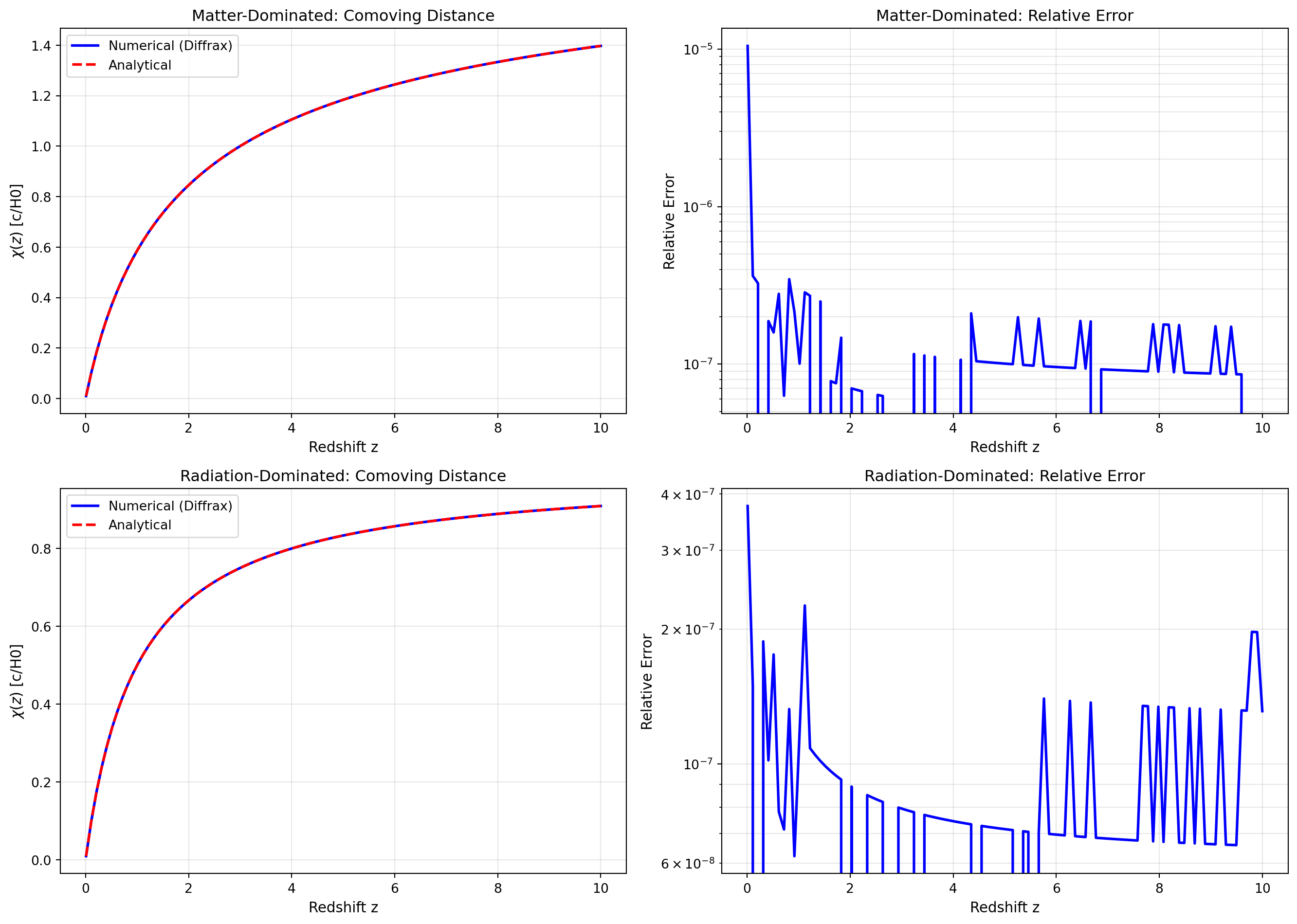

Summary

The numerical integration using Diffrax agrees with the analytical solutions to very high precision (relative errors typically < \(10^{-6}\)). This validates our implementation and demonstrates that:

The ODE formulation correctly represents the cosmological integrals
The Dopri5 solver with adaptive stepping provides excellent accuracy
JAX’s automatic differentiation infrastructure works seamlessly with the ODE solver

The small residual errors are primarily due to:

Finite tolerance settings (rtol=1e-8, atol=1e-10)
Finite starting point for the age integral (log a = -20 instead of -∞)

These can be reduced further by tightening tolerances or starting the age integration at an even earlier time, at the cost of additional computation.