14 The Horizon Problem
We’ve already encountered two interesting puzzles with our standard Big Bang cosmology. The first, although not emphasized, was that the age of the Universe - given only matter and radiation and a Hubble constant close to its value today - is inconsistent with observations.
The second was the flatness problem - \(\Omega_{K}\) being so close to 0 today implies that it must have been vanishingly small in the past. The puzzle is then to dynamically explain where such a small value could come from.
The third is the horizon problem. This is best discussed with a picture of the CMB
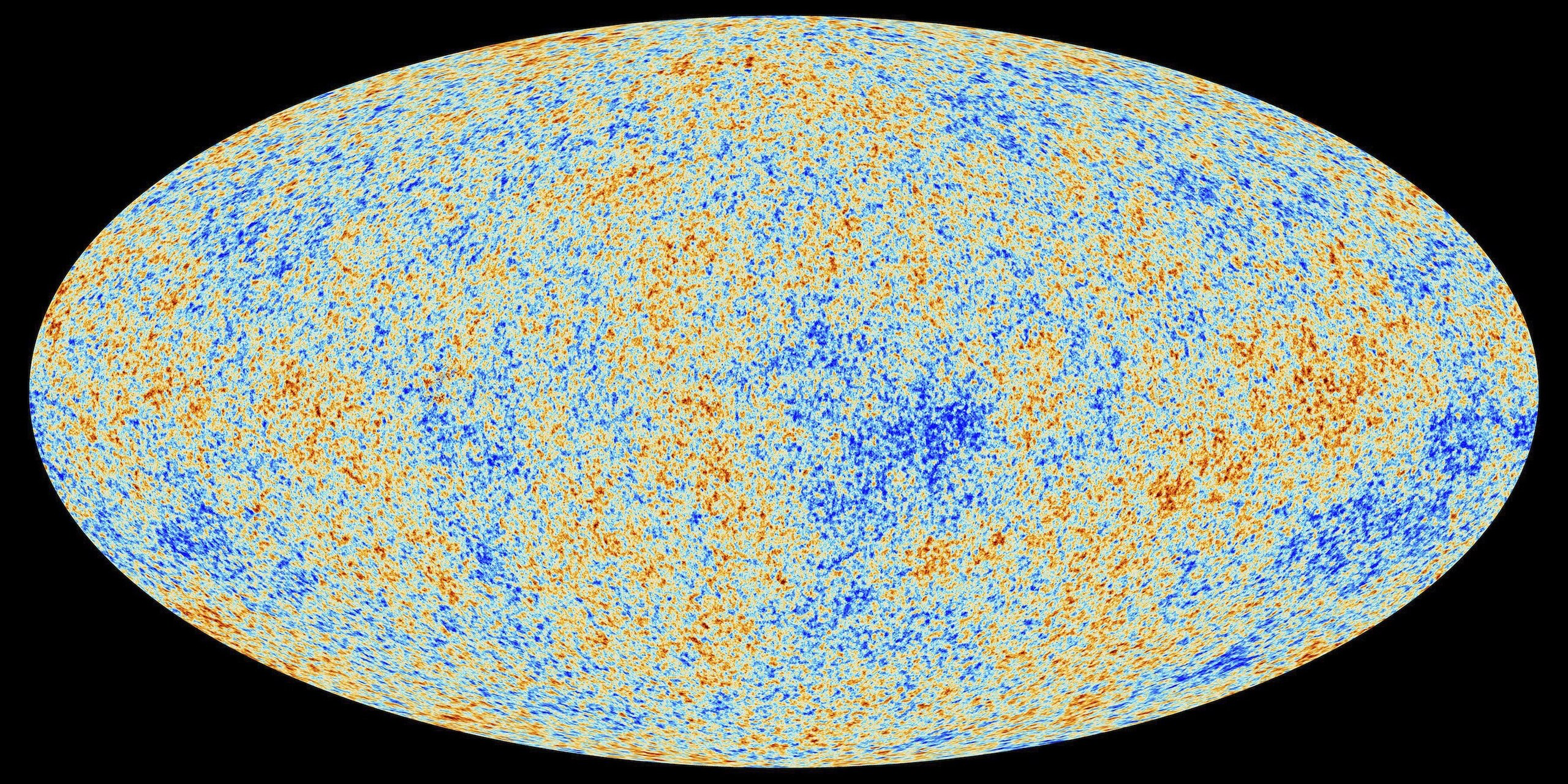
The fluctuations in the above map are a part in \(10^{-5}\); the temperature itself is a uniform 2.73K across the entire sky. However, as we’ll see, different parts of this map have not been in causal contact at the time the CMB was created. So the puzzle is how does one dynamically get such a uniform map across the entire sky.
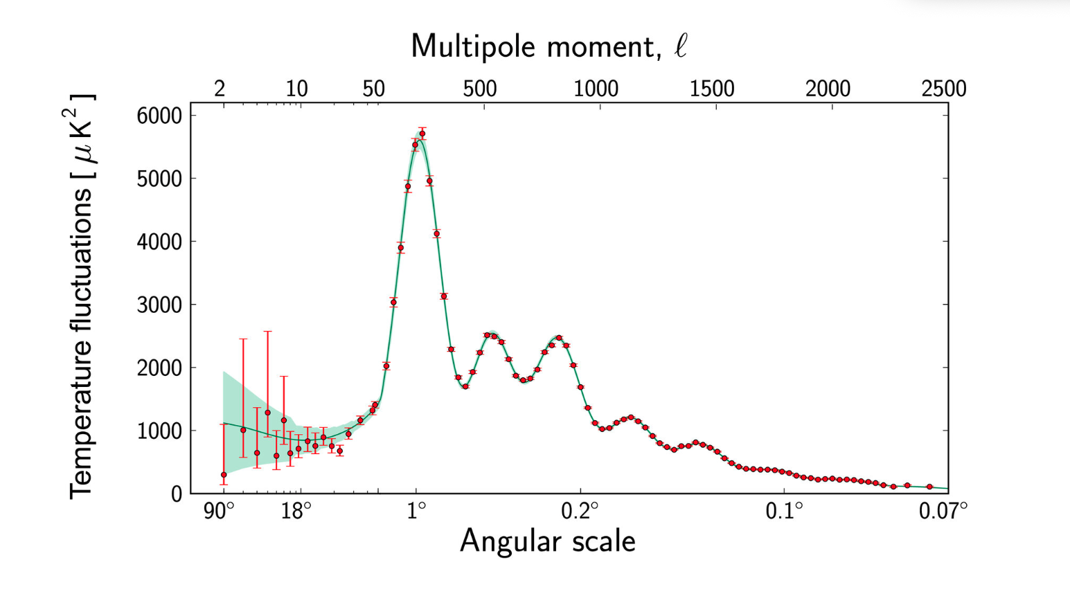
There is a second (and almost even worse) problem. It’s not just that the map is uniform, but it’s also that the fluctuations in the map are actually correlated with one another, best seen in the CMB angular power spectrum shown below.
As we’ll see the solution to all of these is a period of accelerated expansion - or equivalently a period of a decreasing Hubble radius - in time. For the age problem, this is provided by dark energy, while for the horizon and flatness problem, this is solved by inflation.
14.1 Horizons
Before we proceed, it is useful to define different concepts of “horizons” that show up in cosmology. In what follows, it is more elegant and convenient to work in conformal time coordinates \[ ds^{2} = a(t)^{2} \left[ -d \eta^{2} + d\chi^{2} \right] \]
The particle horizon is defined as the region could have causally affected a point. From the metric, we see that the particle horizon is defined by \[ \chi_{p} = \eta - \eta_{i} = \int_{t_{i}}^{t} \frac{1}{a(t)} \, dt \] where \(\eta_{i}\) is our initial time. The particle horizon is what is most relevant for our discussion below.
The second horizon is the event horizon, which is the maximal radius out to which we can be in causal contact in the future. The figure below sketches out the ideas of a particle and event horizon.
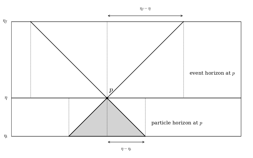
Finally, we have the comoving Hubble radius \((a H)^{-1}\), which is how far a particle could travel “now” (i.e. before the Universe appreciably expands). As we’ll see below, for matter and radiation, \(\chi_{p} \sim (a H)^{-1}\) and the two are often just conflated.
14.2 The Horizon Problem, restated
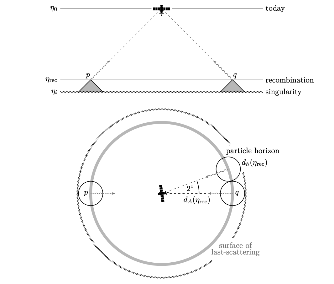
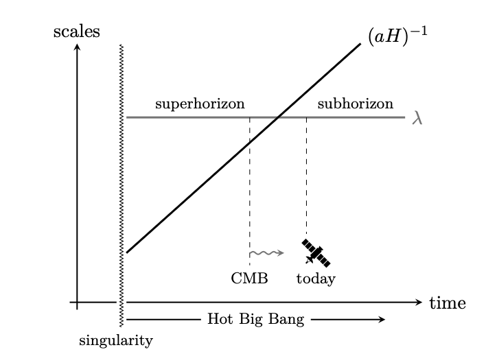
The horizon problem can now be easily restated with the following figure (Fig. 4.2 in Baumann)
We can see the issue in the following. The particle horizon can be written as \[ \chi_{p} = \int_{t_{i}}^{t} \frac{1}{a(t)} \, dt = \int_{a_{i}}^{a} \frac{1}{a \dot{a}} \, da = \int_{\ln a_{i}}^{\ln a} \frac{1}{a H(a)} \, d\ln a \] relating the particle horizon to evolution of the comoving Hubble radius. For normal matter, the comoving Hubble radius is monotonically increasing and so, this integral is dominated by late times, giving rise to the picture above.
We can be more explicit by considering a constant equation of state \(w\). In this case, we have \[ H(a) = H_{0} a^{-3(1+w)/2} \] or \[ (a H)^{-1} = H_{0}^{-1} a^{(1+3w)/2} \] which is clearly monotonically increasing if \(w > -\frac{1}{3}\) (which was our condition for a decelerating Universe). The particle horizon is then \[ \chi_{p}(a) = \eta - \eta_{i} = \frac{2H_{0}^{-1}}{1+3w} \left[ a^{(1+3w)/2} - a_{i}^{(1+3w)/2} \right] \] Note that (for \(w>-\frac{1}{3}\)) \[ a^{(1+3w)/2} \to 0 \text{ as } a \to 0 \] again emphasizing that the particle horizon is dominated by late time contributions.
We can estimate these for \(w=0\). The particle horizon at the CMB \(a \sim 10^{-3}\) is \[ \chi_{CMB} = 2 \times 3000 \times \sqrt{ 0.001} \approx 200 \text{ Mpc/h} \approx 286 \text{ Mpc} \] while the distance to the CMB is \[ r_{CMB} = (6000 - 200) \approx 6000 \text{ Mpc/h} \approx 8600 \text{ Mpc} \] The angle subtended by the particle horizon on the CMB is therefore \(\sim 2^{\circ}\).
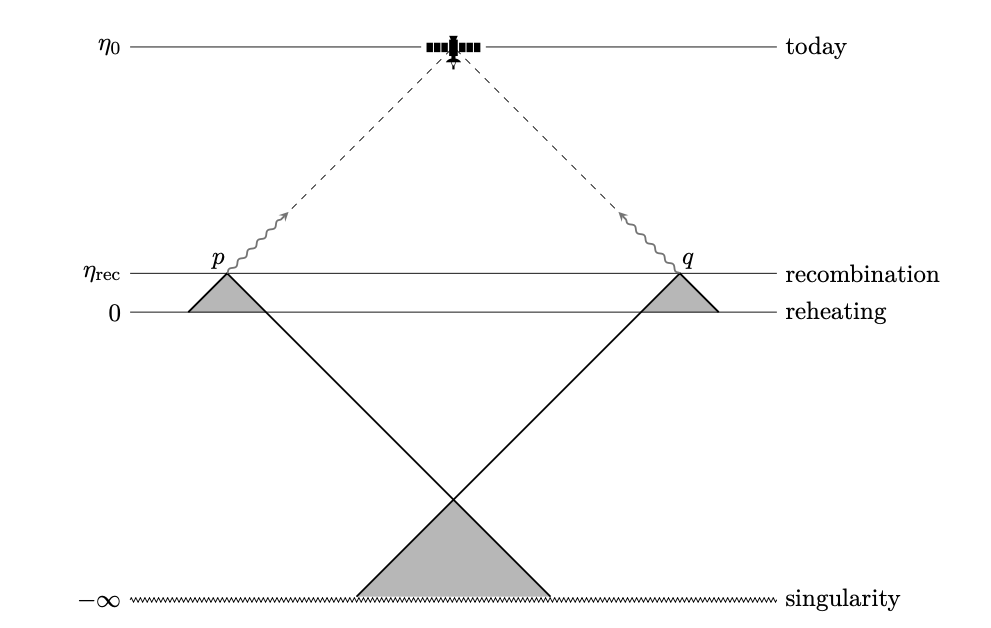
A similar story can be told for the superhorizon correlations seen in the figure below (Fig. 4.3 in Baumann) where a fluctuation of a scale \(\lambda\) is compared with the comoving Hubble radius (which as we see above is similar to the particle horizon for standard matter). However, we see scales in the CMB that are correlated that would have been greater than the particle horizon/Hubble radius at the time of the CMB.
14.3 The Inflationary Solution
One solution to this problem is to introduce a period where the Hubble radius is shrinking with time. We can do this in our simple model with a period (referred to as inflation) dominated by a component with \(1+3w < 0\) or \(w < -1/3\). In this case, we have \[ \eta_{i} \to -\infty \text{ as } a_{i} \to 0 \] giving us plenty of time to bring regions into causal contact. This is shown in the figure below (Fig 4.4 in Baumann). Note that in this picture, the hot Big Bang is not a singularity, but rather just a point in time in the Universe when this inflation ends.
Note that a shrinking Hubble sphere is equivalent to an accelerated expansion of the Universe \[ \begin{aligned} aH &= \dot{a} \\ \frac{d}{dt} (aH)^{-1} < 0 &=> \frac{d}{dt} \frac{1}{\dot{a}} < 0 \\ \ddot{a} &> 0 \end{aligned} \] It is also sometimes referred to as a period of exponential expansion, which is what one gets if \(w \sim -1\) (just as with dark energy).
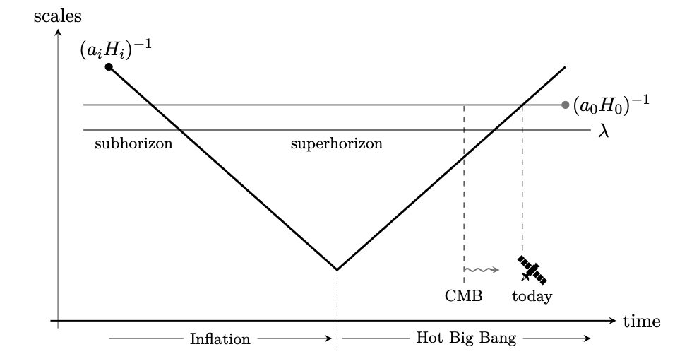
The picture for superhorizon correlations also gets modified to the figure below (Fig. 4.7 in Baumann), where we see a mode start inside the horizon, exit and then re-enter the horizon.
How much inflation?
Let us now estimate how long this period of inflation would need to be. A simple condition for inflation to work is that \[ (a_{0} H_{0})^{-1} < (a_{i} H_{i}) \] i.e. that the comoving Hubble radius today is less than the comoving Hubble radius at the start of inflation. As before, today will be denoted by \(0\), while the start of inflation will be \(i\). We will also denote the end of inflation (which is the “hot Big Bang”, or the reheating epoch) as \(e\).
For simplicity, we will just consider \(w=-1\) to describe the inflationary epoch. This implies \(H_{e} = H_{i}\). Furthermore, let us just imagine the Universe post reheating/inflation was just radiation dominated and so \(H \propto a^{-2}\). This gives us \[ \frac{a_{0} H_{0}}{a_{e} H_{e}} = \frac{a_{0}}{a_{e}} \left( \frac{a_{e}}{a_{0}} \right)^{2} = \frac{a_{e}}{a_{0}} \sim \frac{T_{0}}{T_{e}} \sim 10^{-28} \left( \frac{10^{15} \text{ GeV}}{T_{e}} \right) \] Now define the number of e-folds of inflation \[ N = \ln\left( \frac{a_{e}}{a_{i}} \right) \] our condition becomes \[ \begin{aligned} \frac{a_{i} H_{i}}{a_{0} H_{0}} > 1 \\ e^{-N} \frac{a_{e} H_{e}}{a_{0} H_{0}} > 1 \\ N > 64 + \ln\left( \frac{T_{e}}{10^{15} \text{ GeV}} \right) \end{aligned} \]
Flatness Revisited
We can now see whether this same solution addresses the flatness problem. Suppose at the start of inflation, the Universe had some non-zero \(\Omega_{K,i}\). At the end of inflation, we have \[ \Omega_{K,e} \sim \Omega_{K,i} \left( \frac{a_{i}}{a_{e}} \right)^{-2} \] since \(H\) is approximately constant. From our previous estimate, this gives \[ \Omega_{K,e} \sim \Omega_{K,i} e^{-2 N} \] Inflation drives down the curvature to a negligible value.