Code
import jax
import jax.numpy as jnp
from jax import grad, vmap
import diffrax
import matplotlib.pyplot as pltAs a simple example of computing a Fisher matrix and estimating parameter errors in a cosmological context, we consider the following toy problem. Imagine that we measure the comoving distance \(\chi\) (in units of \(c/H_0\)) at a single redshift with a known measurement error \(\sigma_\chi\). We’ll assume a simple cosmological model with only \(\Omega_m\), and we’d like to estimate the Fisher matrix and the expected error on \(\Omega_m\) from this single measurement.
In this case, the derivatives are analytically tractable, so you could compute the Fisher matrix with standard numerical integration. However, as a demonstration, we will continue to explore differentiable programming and compute the Fisher matrix using automatic differentiation. See previous notebooks for examples of using JAX for automatic differentiation in cosmology.
Let’s just write down the Fisher matrix for this simple case.
The general form of the Fisher matrix for a fixed covariance matrix \(C\) and a model \(\mu\) is \[ F_{ij} = \frac{\partial \mu^T}{\partial \theta_i} C^{-1} \frac{\partial \mu}{\partial \theta_j} \] where \(\theta_i\) are the model parameters (in our case, just \(\Omega_m\)), \(\mu\) is the model prediction for the observable (here, the comoving distance \(\chi\)), and \(C\) is the covariance matrix of the measurement (here, just \(\sigma_\chi^2\)).
In our case, this simplifies to a single parameter and a single measurement, so the Fisher matrix is just a scalar: \[ F = \frac{1}{\sigma_\chi^2} \left( \frac{\partial \chi}{\partial \Omega_m} \right)^2 \] and the expected error on \(\Omega_m\) is simply \[ \sigma_{\Omega_m} = \frac{1}{\sqrt{F}}. \]
import jax
import jax.numpy as jnp
from jax import grad, vmap
import diffrax
import matplotlib.pyplot as pltWe use JAX and Diffrax to compute the comoving distance, following the approach in the Friedmann-Numerical-JAX notebook. The key advantage is that JAX gives us automatic differentiation for free.
# Fiducial cosmology (flat ΛCDM)
Om_fid = 0.3
Ol_fid = 0.7

def EHubble(Om, z):
    """Dimensionless Hubble parameter E(z) = H(z)/H0 for flat ΛCDM."""
    Ol = 1.0 - Om  # Flat universe
    return jnp.sqrt(Om * (1 + z)**3 + Ol)

def comoving_radial_distance(Om, z_final, rtol=1e-8, atol=1e-10):
    """Comoving radial distance χ(z) in c/H0 units using Diffrax ODE solver."""

    def dchi_dz(z, chi, args):
        """ODE: dχ/dz = 1/E(z)"""
        return 1.0 / EHubble(Om, z)

    term = diffrax.ODETerm(dchi_dz)
    solver = diffrax.Dopri5()
    stepsize_controller = diffrax.PIDController(rtol=rtol, atol=atol)

    sol = diffrax.diffeqsolve(
        term, solver,
        t0=0.0, t1=z_final, dt0=0.01, y0=0.0,
        stepsize_controller=stepsize_controller,
    )
return sol.ys[0]Now we use JAX’s automatic differentiation to compute \(\partial \chi / \partial \Omega_m\). The Fisher error on \(\Omega_m\) is then: \[ \sigma_{\Omega_m} = \frac{\sigma_\chi}{|\partial \chi / \partial \Omega_m|} \]
We’ll assume a fixed fractional error on the distance measurement, say 1%.
# Compute derivative of χ with respect to Ωm
dchi_dOm = grad(comoving_radial_distance, argnums=0)

# Measurement error: assume 1% fractional error on distance
fractional_error = 0.01

def fisher_error_Om(Om, z):
    """Compute the Fisher error on Ωm from a distance measurement at redshift z."""
    chi = comoving_radial_distance(Om, z)
    deriv = dchi_dOm(Om, z)
    sigma_chi = fractional_error * chi
    # σ_Ωm = σ_χ / |∂χ/∂Ωm|
    return sigma_chi / jnp.abs(deriv)

# Test at a few redshifts
z_test = jnp.array([0.5, 1.0, 2.0, 3.0])
print("Fisher error on Ωm from 1% distance measurement:")
print("=" * 50)
print(f"{'z':>8} {'χ [c/H0]':>12} {'∂χ/∂Ωm':>12} {'σ(Ωm)':>12}")
print("-" * 50)
for z in z_test:
    chi = comoving_radial_distance(Om_fid, z)
    deriv = dchi_dOm(Om_fid, z)
    sigma_Om = fisher_error_Om(Om_fid, z)
    print(f"{z:8.1f} {chi:12.4f} {deriv:12.4f} {sigma_Om:12.4f}")
Fisher error on Ωm from 1% distance measurement:
==================================================
z χ [c/H0] ∂χ/∂Ωm σ(Ωm)
--------------------------------------------------
0.5 0.4410 -0.1529 0.0288
1.0 0.7714 -0.4577 0.0169
2.0 1.2095 -1.0380 0.0117
3.0 1.4840 -1.4596 0.0102Let’s plot how the constraining power on \(\Omega_m\) changes with the redshift of the measurement. Higher redshift measurements probe larger distances where the sensitivity to \(\Omega_m\) is greater.
# Compute Fisher error over a range of redshifts
z_range = jnp.linspace(0.1, 5.0, 50)
fisher_error_vec = vmap(lambda z: fisher_error_Om(Om_fid, z))
sigma_Om_vals = fisher_error_vec(z_range)

# Also compute the derivative for reference
deriv_vec = vmap(lambda z: dchi_dOm(Om_fid, z))
deriv_vals = deriv_vec(z_range)

# Create figure
fig, (ax1, ax2) = plt.subplots(1, 2, figsize=(12, 5))

# Left panel: Fisher error
ax1.plot(z_range, sigma_Om_vals, 'b-', linewidth=2)
ax1.set_xlabel('Redshift $z$', fontsize=12)
ax1.set_ylabel(r'$\sigma_{\Omega_m}$', fontsize=12)
ax1.set_title(r'Fisher Error on $\Omega_m$ (1% distance error)', fontsize=12)
ax1.grid(True, alpha=0.3)
ax1.set_ylim(bottom=0)

# Right panel: derivative (sensitivity)
ax2.plot(z_range, jnp.abs(deriv_vals), 'r-', linewidth=2)
ax2.set_xlabel('Redshift $z$', fontsize=12)
ax2.set_ylabel(r'$|\partial \chi / \partial \Omega_m|$ [c/H$_0$]', fontsize=12)
ax2.set_title(r'Sensitivity of Distance to $\Omega_m$', fontsize=12)
ax2.grid(True, alpha=0.3)

plt.tight_layout()
plt.show()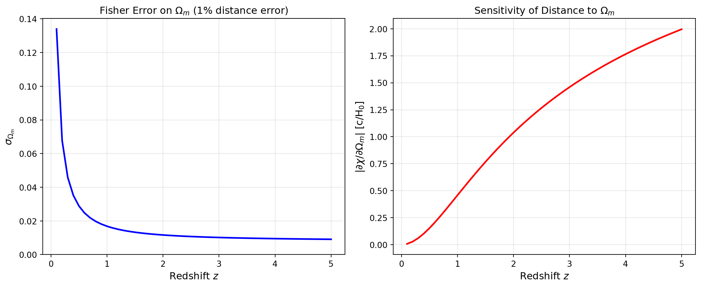
The plots show that:
Of course, this is a simplified example. Real surveys must account for: