22 Neutrinos in Cosmology - I
22.1 Preface
Just a note on these lectures - these are not part of our regular development, but are additional lectures written for PHYS6600. They are therefore intended to be more standalone lectures and will repeat some of the material in other parts of the course.
The lectures here largely follow Baumann’s textbook closely with some commentary interspersed.
I plan for these lectures to roughly follow three broad themes:
- Relativistic Neutrinos (and other species) - Equilibrium thermodynamics in the Early Universe.
- The Boltzmann equation - freezing out of particles; WIMP freeze out and other examples.
- Massive Neutrinos - measuring the neutrino mass through large scale structure.
22.2 A Brief Review of Cosmology
Overview
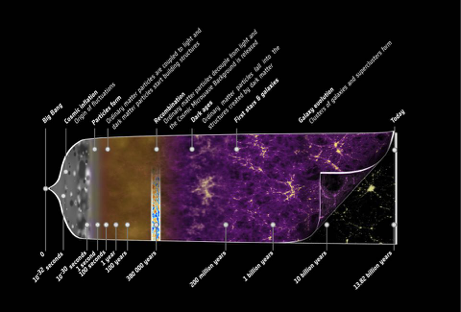
The figure above is an overview of the entire history of the Universe, from the Big Bang to today. Neutrinos play a role in this picture throughout, but especially in two epochs - the early radiation dominated epoch where they are effectively massless and help determine the expansion rate of the Universe. And their second act is at late times, when they transition to non-relativistic matter and act as warm dark matter. This first lecture focuses on the first of these.
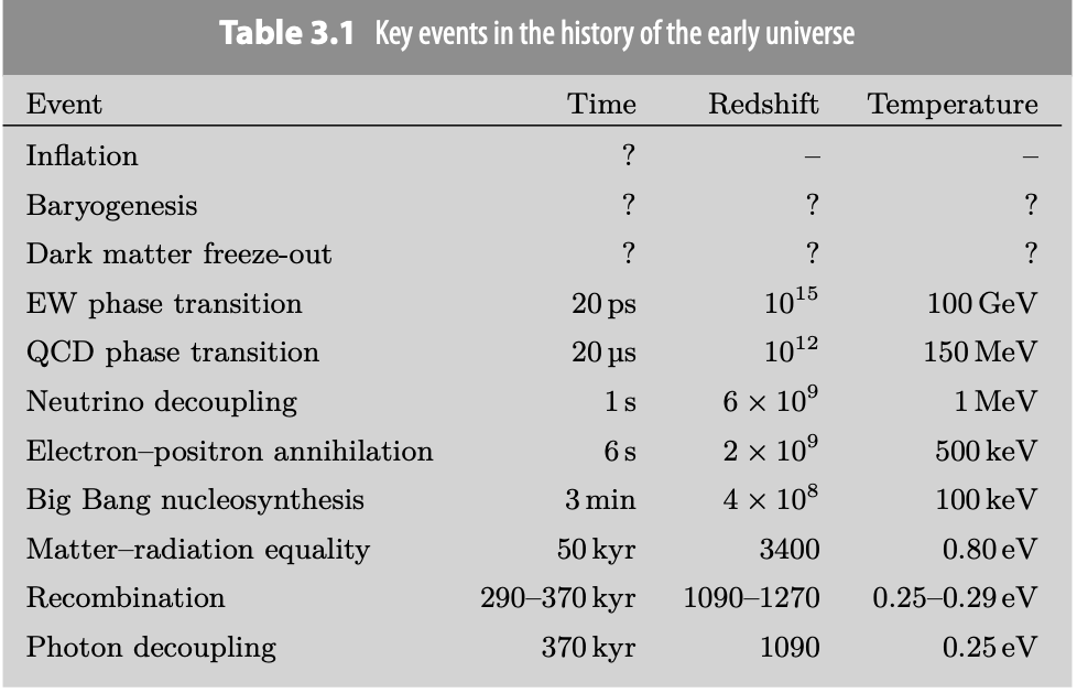
The table below highlights some key times in the history of the Universe. This lecture will largely focus on the times \(< 10\)s after the Big Bang/inflation, when the temperature drops down to \(\sim 500\) keV, just below the rest mass of the electron. The imprints of these will be seen both in BBN as well as the CMB.
The Friedmann Universe
In all of what follows, we will use natural units \(c = \hbar = 1\).
When we describe our Universe, we often break it into a homogeneous expansion, and the effects of small perturbations on this homogeneous expansion. We’ll do the same here today, and for the first set of lectures, we’ll focus in on the homogeneous Universe. We describe our expanding Universe by a scale factor \(a(t)\) which measures the size of the Universe relative to its size today. The redshift is given by \[ 1+z = \frac{1}{a} \]
The Hubble parameter measures the expansion rate as is defined by \[ H = \left( \frac{\dot{a}}{a} \right) \] with a value today of \(H_{0} \approx 70\) km/s/Mpc. Cosmologists often parametrize the remaining uncertainty in this value by writing \(H_{0} = 100h\) km/s/Mpc, which results in factors of \(h\) in expressions.
The expansion rate is determined by the energy density in the Universe. This is described by the Friedmann equation \[ \left(\frac{\dot{a}}{a}\right)^{2} = \frac{8 \pi G}{3} \rho(t) - \frac{k}{R_0^{2} a^{2}} \] and the continuity equation \[ \dot{\rho} + 3 H (\rho + P) = 0 \] where the latter differs from the regular continuity equation due to the expansion history of the Universe.
Given an equation of state, the continuity equation allows us to describe the evolution of different components of the Universe. In cosmology, we assume a simple equation of state of the form \(P = w \rho\). We have the following cases that are important…
- Pressure-less Matter/Dust
\[ w=0 \implies \rho = \rho_{0}a^{-3} \]
- Radiation \[ w = \frac{1}{3} \implies \rho = \rho_{0} a^{-4} \]
- Cosmological Constant \[ w = -1 \implies \rho = \rho_{0} \]
We can put this together a single figure that shows the evolution of each of these terms with scale factor:
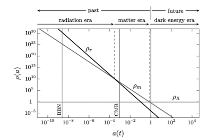
Finally, we note that \(T \propto a^{-1}\) (at least away from particle masses, we’ll see a more accurate version later). What this means is that for the period of interest today, the Universe will be radiation dominated, and the Friedmann equation becomes \[ H^{2} = \frac{\rho}{3 M_{pl}^{2}} \] where \[ M_{pl}^{2} \equiv \frac{\hbar c}{8 \pi G} = 2.4 \times 10^{18} \, \text{GeV} \]
We will also sometimes talk about densities relative to the critical density \[ \rho_\text{crit} = \frac{3H^{2}}{8 \pi G} \] Note that the value of the critical density depends on \(H\) and therefore varies with time. The value today is \[ \begin{aligned} \rho _\text{crit} &= 1.877 \times 10^{-26} h^{2} \text{kg}\,\text{m}^{-3} \\ &= 2.775 \times 10^{11} h^{2} M_{\odot} \text{Mpc}^{-3} \\ &= 1.053 \times 10^{10} \text{eV}^{4} \end{aligned} \]
We can measure the density relative to the critical density \[ \Omega = \frac{\rho}{\rho _\text{crit}} \]
22.3 A Brief Review of Thermodynamics
Since we’re talking about the thermal history of the Universe, recall some key results from thermodynamics/statistical mechanics. We’ll assume equilibrium throughout, so will assume a temperature \(T\). All of the results here can be derived by starting from either the Bose-Einstein or Fermi-Dirac equations and integrating over the density of states.
A relativistic gas of a species with negligible chemical potential has a number density \[ n = \frac{\zeta(3)}{\pi^{2}} g T^{3} \begin{cases} 1 & \text{bosons} \\ \frac{3}{4} & \text{fermions} \end{cases} \] where \(g\) is the number of internal degrees of freedom it has. We get a analogous relation for the density
\[ \rho = \frac{\pi^{2}}{30} g T^{4} \begin{cases} 1 & \text{bosons} \\ \frac{7}{8} & \text{fermions} \end{cases} \] and the pressure in the relativistic regime is given by \[ P = \frac{\rho}{3} \] Note that the density evolves as \(\rho \propto T^{4}\) which is consistent with our previous scaling with radiation. We should note here that radiation includes all relativistic particles - photons, neutrinos and as we go back in time, all standard model particles.
As an exercise, we can use the above to calculate the number density and energy density of the CMB photons today. Using \(T_\text{CMB} \approx 2.73 \,K\), we can plug in to the above and find \[ \begin{aligned} n_{\gamma,0} & \approx 410 \,\text{photons}\,\text{cm}^{-3} \\ \rho_{\gamma,0} & \approx 4.6 \times 10^{-34} \,\text{g}\,\text{cm}^{-3} \\ \Omega_{\gamma} h^{2} &\approx 2.5 \times 10^{-5} \end{aligned} \]
In the non-relativistic limit, we find \[ n = g \left( \frac{mT}{2\pi} \right)^{3/2} e^{-m/T} \] and \[ \rho \approx m n + \frac{3}{2} n T \]
\[ P = n T \approx 0 \] For our purposes today, this means that as a particle goes non-relativistic, its number density is exponentially suppressed and it quickly becomes irrelevant. This statement is only true in equilibrium - we will return to this later.
22.4 Counting States - I
Given the above, understanding the expansion history of the Universe during radiation domination is therefore just a matter of accounting for all the relativistic species \[ \rho = \sum_{i} \rho_{i} \] It is convenient to write this as \[ \rho = \frac{\pi^{2}}{30} g_{*}(T) T^{4} \] where we have defined an effective number of states \[ g_{*}(T) = \sum_{i=\text{bosons}} g_{i} \left( \frac{T_{i}}{T} \right)^{4} + \frac{7}{8} \sum_{i=\text{fermions}} g_{i} \left( \frac{T_{i}}{T} \right)^{4} \] In the above, we allow for the possibility that different species have different temperatures, which is possible when they decouple from the overall thermal bath. The temperature \(T\) is the common temperature of the rest, often just assumed to be the photon temperature. In the standard model, this effect is only relevant for neutrinos, which decouple the first, since they have the weakest cross section.
We can now go ahead and count internal degrees of states. The two tables below (taken from Baumann) describe the particle content of the standard model, highlighting the masses of the particles as well as their spin. When \(T_{i} \gg m\), the particles will be relativistic and will contribute to the overall radiation density of the Universe. In the opposite limit (assuming the particles are still in equilibrium), the particles rapidly annihilate and their number density is exponentially suppressed. Note that this assumes equilibrium, which is true for our story today. However, non-equilibrium effects play a critical role in the number density calculations and we’ll turn to these in the next lecture.
Some rules here:
- Massless particles with spin have two polarization states.
- Massive particles of spin \(s\) has \(2s+1\) polarization states.
- Count both particles and anti-particles.
- Quarks have 3 colors, while there are 8 gluons.
| Type | Particle | Mass | Spin | \(g\) |
|---|---|---|---|---|
| gauge bosons | \(\gamma\) | 0 | 1 | 2 |
| \(W^\pm\) | 80 GeV | 1 | 3 | |
| \(Z\) | 91 GeV | |||
| gluons | \(g_i\) | 0 | 1 | \(8 \times 2 = 16\) |
| Higgs boson | \(H\) | 125 GeV | 0 | 1 |
| quarks | \(t, \bar{t}\) | 173 GeV | \(\frac{1}{2}\) | \(2 \times 3 \times 2 = 12\) |
| \(b, \bar{b}\) | 4 GeV | |||
| \(c, \bar{c}\) | 1 GeV | |||
| \(s, \bar{s}\) | 100 MeV | |||
| \(d, \bar{d}\) | 5 MeV | |||
| \(u, \bar{u}\) | 2 MeV |
| Particle | Mass | Spin | \(g\) |
|---|---|---|---|
| \(\tau^\pm\) | 1777 MeV | \(\frac{1}{2}\) | \(2 \times 2 = 4\) |
| \(\mu^\pm\) | 106 MeV | ||
| \(e^\pm\) | 511 keV | ||
| \(\nu_\tau, \bar{\nu}_\tau\) | \(< 0.6\) eV | \(\frac{1}{2}\) | \(2 \times 1 = 2\) |
| \(\nu_\mu, \bar{\nu}_\mu\) | \(< 0.6\) eV | ||
| \(\nu_e, \bar{\nu}_e\) | \(< 0.6\) eV |
Of course, the story for neutrinos is more complicated. If they were massless, then this would be easy. However, if they have mass, then we need to decide on what type of mass - a Majorana or Dirac mass. For our purposes, the important piece here is that is neutrinos had a Majorana mass, they would be their own anti-particle, and so would not get an additional factor of 2 from that. If they are Dirac particles, then you would get an additional factor of 2, and neutrino measurements would be inconsistent with BBN. The way out would be to have half of these degrees decouple in the very early Universe and then dilute away. Determining the mass type is still an open question.
Adding up internal degrees of freedom, we find
- \(g_{b} = 28\) : photons(2), \(W^{\pm}\) and \(Z\) (3x3), gluons (8x2) and Higgs (1)
- \(g_{f} =90\) : quarks (6x12), charged leptons (3x4), neutrinos (3x2)
Putting this together, we get \[ g_{*} = g_{b} + \frac{7}{8} g_{f} = 106.75 \]
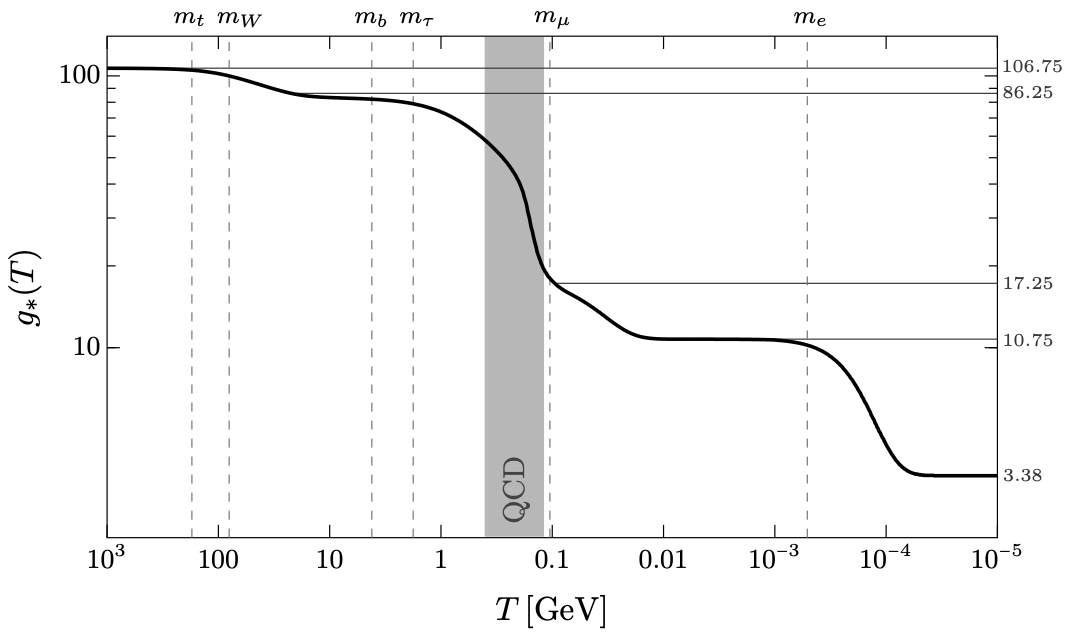
As the temperature of the Universe decreases, various species go non-relativistic and drop out from \(g_{*}\). This continues until the charm quark. At this point, the QCD phase transition takes place and the quarks get bound up into baryons and mesons, of which only the pions are light enough to contribute here. These are spin 0, and so carry a total of 3 internal degrees of freedom, resulting in a total of \(g_{*}=17.25\). Soon after this, muons and pions annihilate with \(g_{*}\) dropping to 10.75.
At this point, electrons and protons will annihilate, and the neutrinos will decouple. However, to fully understand that, we need to discuss the evolution of entropy.
22.5 Entropy
Let’s start with the first law of thermodynamics (in the absence of a chemical potential) \[ T dS = dU + P dV \] Rewriting this in terms of the entropy \(s\) and energy density \(\rho\), we have \[ \begin{aligned} T d(sV) = d(\rho V) + P dV \\ TV ds + Ts dV = \rho dV + V d\rho + P dV \\ (Ts - \rho - P) dV + V\left( T \frac{ds}{dT} - \frac{d\rho}{dT} \right) dT = 0 \end{aligned} \] Since this must be true for all variations \(dV\) and \(dT\), we have \[ s = \frac{\rho + P}{T} \] and \[ \frac{ds}{dT} = \frac{1}{T} \frac{d\rho}{dT} \] Using the continuity equation \[ \frac{d\rho}{dt} = -3 H(\rho + P) = -3 H T s \] we get \[ \frac{d(s a^{3})}{dt} = 0 \] or the statement that the total entropy is conserved in the Universe, and \(s \propto a^{-3}\).
We can also write out an expression for \(s\) \[ s = \sum_{i} \frac{\rho_{i}+P_{i}}{T_{i}} = \frac{2\pi^{2}}{45} g_{*,S}(T) T^{3} \] where \[ g_{*,S}(T) \approx \sum_{i=\text{bosons}} g_{i} \left( \frac{T_{i}}{T} \right)^{3} + \frac{7}{8} \sum_{i=\text{fermions}} g_{i} \left( \frac{T_{i}}{T} \right)^{3} \] away from mass thresholds. Note the similarities and differences with \(g_{*}\); if all species have a common temperature, then \(g_{*} = g_{*,S}\).
A consequence of entropy conservation is \[ g_{*,S}(T) T^{3} a^{3} = \text{constant} \] We can also plug this in to the Friedmann equation - here we just note that at about 1s, the Universe was \(T = 1\) MeV, and evolves as \(t^{-1/2}\) before that.
22.6 Counting States - II : \(e^{\pm}\) annihilation and Neutrino Temperature
At 1 MeV, neutrinos decouple, and soon after, electron-positron annihilation takes place. The energy from \(e^{\pm}\) annihilation gets deposited into the photons but not the neutrinos, raising the photon temperature relative to the neutrino temperature.
We can calculate this effect by using the conservation of entropy. We have \[
g_{*,S} = \begin{cases}
2 + \frac{7}{8} \times 4 = \frac{11}{2} & T > m_{e} \\
2 & T < m_{e}
\end{cases}
\] which raises the photon temperature by a factor of a factor of \((11/4)^{1/3}\). We therefore have \[
T_{\nu} = \left( \frac{4}{11} \right)^{1/3} T_{\gamma} \approx 1.9 \text{K}
\] 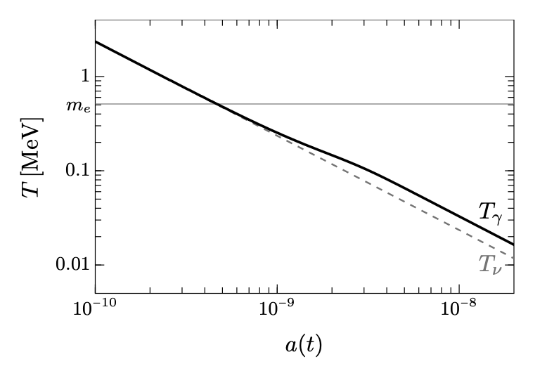
Furthermore, we can calculate the number of degrees of freedom, and we find \[ g_{*} = 2 + \frac{7}{8} \times 2N_{eff} \left( \frac{4}{11} \right)^{1/3} = 3.36 \] Note that the actual value of \(N_{eff}=3.046\), accounting for the fact that neutrino decoupling is not instantaneous and some energy from \(e^{\pm}\) annihilation gets deposited into the neutrinos.
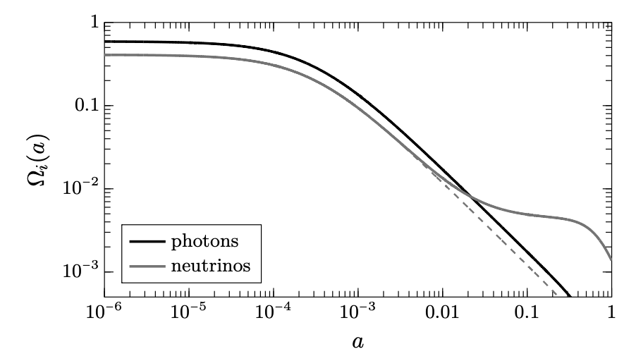
Finally, we can end with plotting the energy density of photons and neutrinos as a function of time. As we see, they largely track each other until low redshift, where the neutrinos go non-relativistic and behave like ordinary matter. But that’s a different discussion.
22.7 Additional Relativistic Species
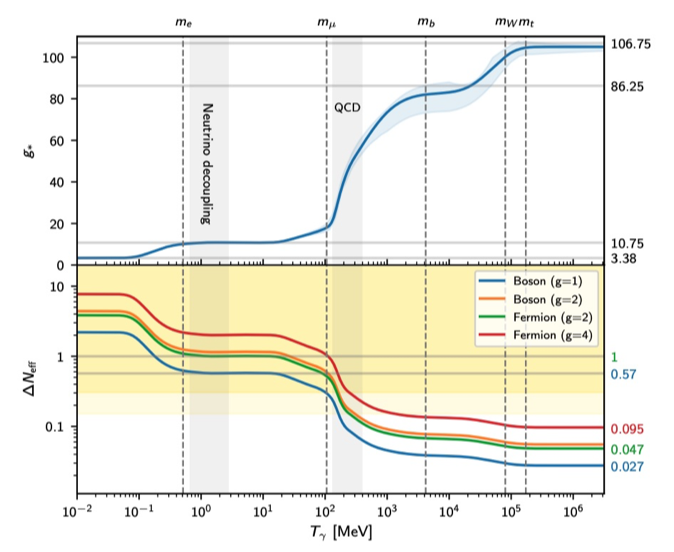
Similar to the neutrino decoupling case, we have \[ T_{X} = \left( \frac{g_{*}(T_{dec,\nu})}{g_{*}(T_{dec,X})} \right)^{1/3} T_{\nu} = 0.465 \left( \frac{106.75}{g_{*}(T_{dec,X})} \right)^{1/3} T_{\nu} \] and \[ \Delta N_{eff} = \frac{\rho_{X}}{\rho_{\nu}} = 0.027 g_{*,X} \left( \frac{106.75}{g_{*}(T_{dec,X})} \right)^{4/3} \]
The figure above, taken from the Planck 2018 cosmological parameters paper shows the \(\Delta N_\text{eff}\) contribution from different particle species as a function of when they decouple.
22.8 Probes
We’ll consider three probes here : Big-Bang Nucleosynthesis, the CMB and baryon acoustic oscillations. A full treatment of these is beyond our scope here, but there are references below for more details.
BBN
The abundance of elements - in particular, helium and deuterium are set by the neutron-proton ratio. We’ll return to a more formal way to calculate this later, but protons and neutrons are coupled to each other by \(\beta\) and inverse-\(\beta\) decay: \[ \begin{aligned} n + \nu_{e} & \leftrightarrow p^{+} + e^{-} \\ n + e^{+} & \leftrightarrow p^{+} + \bar{\nu}_{e} \end{aligned} \]
While the weak interactions are relevant, the neutron to proton ratio is exponentially suppressed by the small mass difference between them and the neutron fraction rapidly falls. However, when the expansion rate is of the same order as the interaction cross-section, the neutron density freezes out, as the figure below shows.
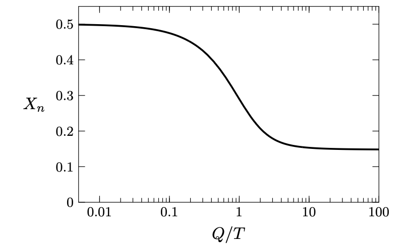 These neutrons will either decay, or get bound into deuterium and then to helium. Since this residual abundance is set by the expansion rate, which is turn is set by the number of relativistic species, the observed helium and deuterium abundances can constrain \(N_{eff}\).
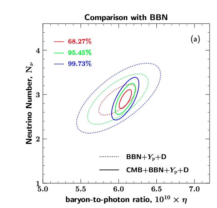
The figures here are from Yeh, Shelton et al, 2022. BBN depends both on the expansion rate, but also the baryon to photon ratio \(\eta\) - the figure below shows the joint constraints on \(N_\text{eff}\) and \(\eta\). The CMB is very effective at constraining \(\eta\) and so breaks much of the degeneracies.
A note on the cases presented. The CMB damping tail (as we’ll discuss below) depends on the helium abundance \(Y_{p}\). The standard CMB analyses use the BBN relationship to determine this value, but one can marginalize out this value as well. We’ll refer to this as the CMB+BBN case, on top of which one can add the measurements of helium and deuterium.
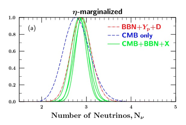
The figure below marginalizes out the value of \(\eta\), X here is none, \(Y_{p}\), \(D\), and \(Y_{p}+D\).
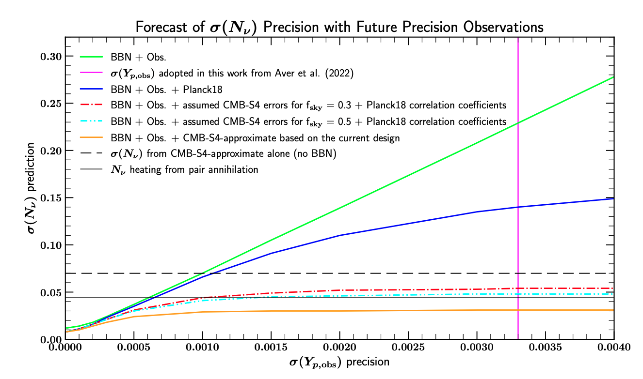
Finally, the figure below shows forecasts as a function of possible future measurements including improved measurements of the helium abundance. The target from \(e^{\pm}\) is shown as a gray line.
CMB
- Primary effect is through the epoch of matter radiation equality
- Secondary effects from damping
- Complicated degeneracies with other parameters.
- Phase shift gives a unique view onto neutrinos.
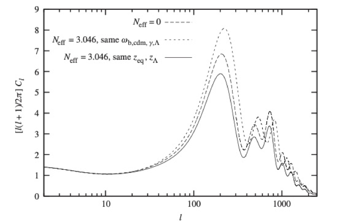
Since the neutrinos contribute non-negligibly to the radiation density of the Universe, they play a significant role in many of the features of the CMB, as this figure from Lesgourges et al, 2013 shows.
One can however introduce \(N_\text{eff}\) as a parameter into the model and constrain it simultaneously with other parameters, the result of which is shown below (from the Planck 2018 results).
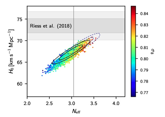
The overall results in that paper are
- \(N_{\text{eff}} = 3.00^{+0.57}_{-0.53}\) (95%, Planck TT+lowE),
- \(N_{\text{eff}} = 2.92^{+0.36}_{-0.37}\) (95%, Planck TT,TE,EE+lowE),
- \(N_{\text{eff}} = 3.11^{+0.44}_{-0.43}\) (95%, TT+lowE+lensing+BAO)
- \(N_{\text{eff}} = 2.99^{+0.34}_{-0.33}\) (95%, TT,TE,EE+lowE+lensing+BAO).
for different cuts through the data and combinations with external data sets.
The two figures below are from Follin et al, 2015, where they detect a phase shift in the CMB acoustic peaks and argue that this is orthogonal from the other effects of neutrinos on the CMB. We reproduce their argument below.
They start by noting that the neutrino background plays a critical role in setting the sound horizon, which in turn sets the scale of the acoustic peaks in the CMB. However, this physical scale isn’t directly measurable, since the distance to the CMB is uncertain due to dark energy in the early Universe (although low redshift measures of the expansion history can help break this degeneracy). Therefore the key observable in the CMB is the angular scale of the acoustic peaks, and this is kept constant in all panels and across all variations (as is the baryon density and baryon to photon ratio, both of which are equally well measured and insensitive to the number of neutrino species). The dominant effect is then the damping of the higher acoustic peaks, seen in the top panel of the figure below.
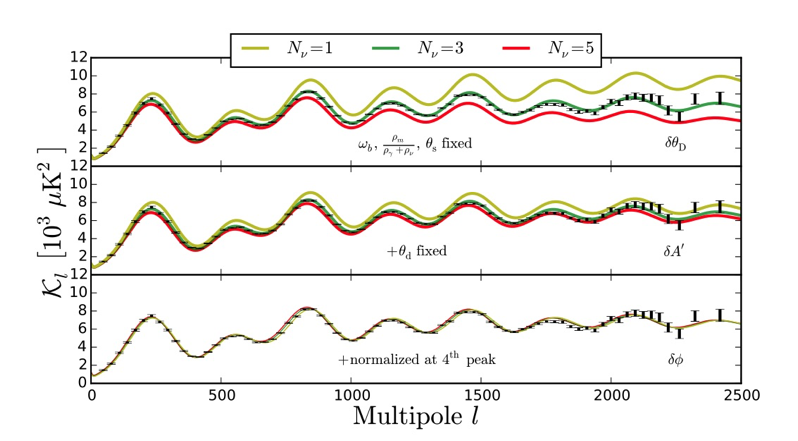
However, this damping scale can be adjusting by changing the helium fraction, giving rise to the second panel. The most noticeable effect is now the an amplitude shift, which is normalized away in the final panel. What we are left with is a phase shift in the acoustic peaks, which can be understood from how neutrino perturbations affect the gravitational potential and therefore the driving of the harmonic oscillator.
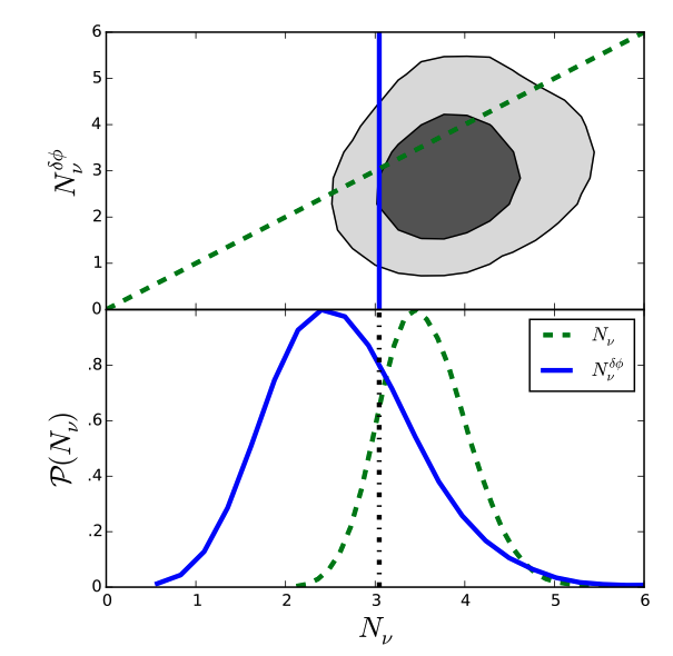
The key point is that neutrinos can change both the amplitude and phase of the acoustic oscillations. The amplitude can be absorbed by many other parameters, but the phase is much more robust. The figure below shows the first detection of this phase, where they allow the \(N_{\nu}\) that drives the gross CMB effects to be separate from the \(N_{\nu}\) that drives the phase. Note that these are both consistent with each other and the expected value that we previously calculated.
BAO
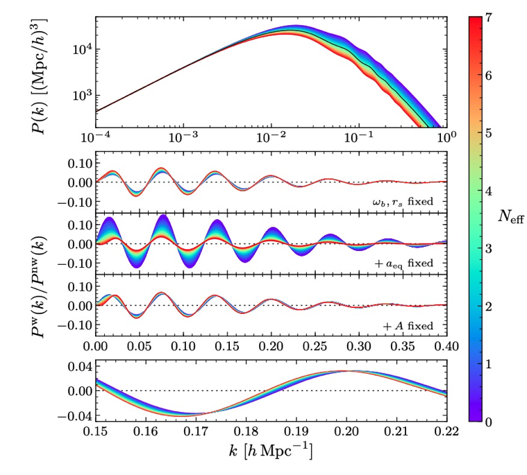
A similar effect can be seen in the galaxy power spectrum. The next two figures (from Baumann et al 2018) highlight the various effects. As with the CMB, there is a residual phase shift that survives even as other physical effects are kept fixed (or marginalized over). The figure below (Fig 3 in the paper) steps through these effects, similar to the CMB discussion above.
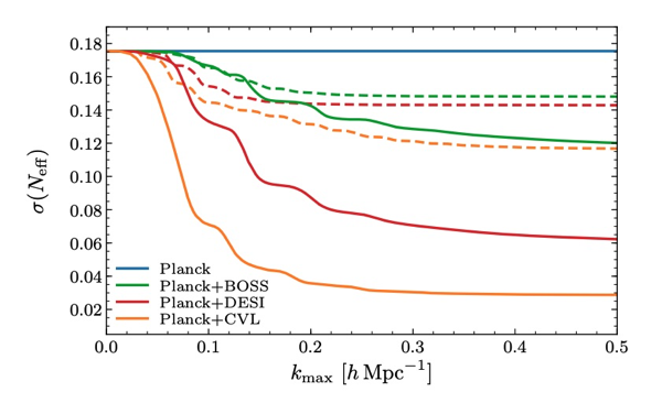
The figure below (Fig 13 in the paper) shows the forecasted sensitivity for both the BAO and galaxy power spectrum for different surveys as a function of the maximum \(k\) scale (the smallest scales that can be reliably used) considered. The dashed lines use just the BAO signal, while the solid line shows the information from the full power spectrum.
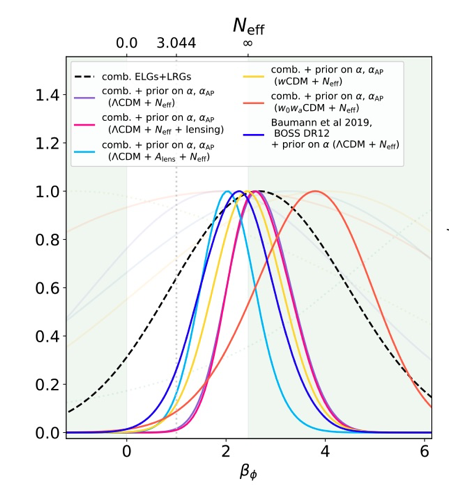
Finally, the figure below from Whitford et al, 2024 shows an initial measurement of this phase shift in the DESI BAO measurements.
22.9 References
- Baumann, Cosmology
- Lesgourges et al, Neutrino Cosmology
- Tsung-Han Yeh et al JCAP10(2022)046
- Follin et al, 1503.07863
- Baumann et al, 1712.08067
- Whitford et al, 2412.05990