Code
import numpy as np
import matplotlib.pyplot as plt
from classy import ClassIn lecture, we sketched out the broad structure of the matter power spectrum in its simplest form. A complete analytic treatment of the full shape of the power spectrum is beyond our scope in this class. However, there are standard codes that allow one to compute these as a function of cosmological parameters.
The two most popular today are CAMB and CLASS. This notebook aims to give you a quick introduction to using CLASS to compute the matter power spectrum and related quantities. CLASS can also be used to compute the CMB power spectra, and we will return to this at the end of this class.
A full description of CLASS, including installation instructions, can be found at the CLASS website. If all you need is the Python interface, you could install it via
pip install classyor a similar equivalent option. As you get more advanced, you might want to install the full CLASS package. (Note that if you are taking ASTR6000, this will already be installed in your Jupyter environment.)
The website also has links to a number of tutorials/course material that go into significantly more detail than we can here. Much of these notes are derived from these.
CLASS has many parameters that can be set, and the simplest documentation of these that I know of is the explanatory input file that it ships with.
You can find this here and I would suggest browsing it.
Let’s compute and plot the matter power spectrum at redshift z=0 using CLASS. Start by importing the necessary libraries.
import numpy as np
import matplotlib.pyplot as plt
from classy import ClassNext, we create an instance of the CLASS class and set the cosmological parameters. The final step will be to call the compute() method to run CLASS.
# Create CLASS instance
cosmo = Class()

# Set cosmological parameters explicitly
cosmo.set({
    'output': 'mPk',           # Request matter power spectrum
    'h': 0.7,                    # Hubble parameter
    'omega_b': 0.02237,        # Baryon density omega_b = Omega_b * h^2
    'omega_cdm': 0.1200,       # CDM density omega_cdm = Omega_cdm * h^2
    'A_s': 2.1e-9,             # Amplitude of primordial power spectrum
    'n_s': 0.9649,             # Spectral index
    'P_k_max_h/Mpc': 50.0,     # Maximum k value in h/Mpc
    'z_max_pk': 0.0            # Maximum redshift for P(k)
})

# Compute
cosmo.compute()

# Print the parameters to check
print("Cosmological parameters set in CLASS:")
print("-----------------------------")
print(f"Omega_b: {cosmo.Omega_b:.5f}")
print(f"Omega_cdm: {cosmo.Omega_cdm:.5f}")
print(f"Omega_m: {cosmo.Omega_m:.5f}")
print(f"h: {cosmo.h:.2f}")
print(f"sigma_8: {cosmo.sigma8:.2f}")
print(f"n_s: {cosmo.n_s:.4f}")
print("-----------------------------")
Cosmological parameters set in CLASS:
-----------------------------
Omega_b: 0.04565
Omega_cdm: 0.24490
Omega_m: 0.29055
h: 0.70
sigma_8: 0.83
n_s: 0.9649
-----------------------------We now have the matter power spectrum computed and can access it via the pk() method. This method takes two arguments: the wavenumber k in units of 1/Mpc, and the redshift z.
# Get k values and power spectrum
# Note: CLASS pk() takes k in 1/Mpc and returns P(k) in Mpc^3
h = cosmo.h
k_h_values = np.logspace(-4, np.log10(50.0), 1000)  # k in h/Mpc
pk_values = np.array([cosmo.pk(k*h, 0.0)*h**3 for k in k_h_values])


# Plot
plt.figure(figsize=(10, 6))
plt.loglog(k_h_values, pk_values, 'b-', linewidth=2)
plt.xlabel(r'$k$ [h/Mpc]', fontsize=14)
plt.ylabel(r'$P(k)$ [(Mpc/h)$^3$]', fontsize=14)
plt.title('Matter Power Spectrum at z=0', fontsize=16)

# Add vertical line for k_eq
k_eq = cosmo.k_eq() / h  # Convert to h/Mpc
plt.axvline(k_eq, color='r', linestyle='--', label=r'$k_{eq}$')
plt.legend()

plt.grid(True, alpha=0.3)
plt.tight_layout()
plt.show()

# Clean up
cosmo.struct_cleanup() 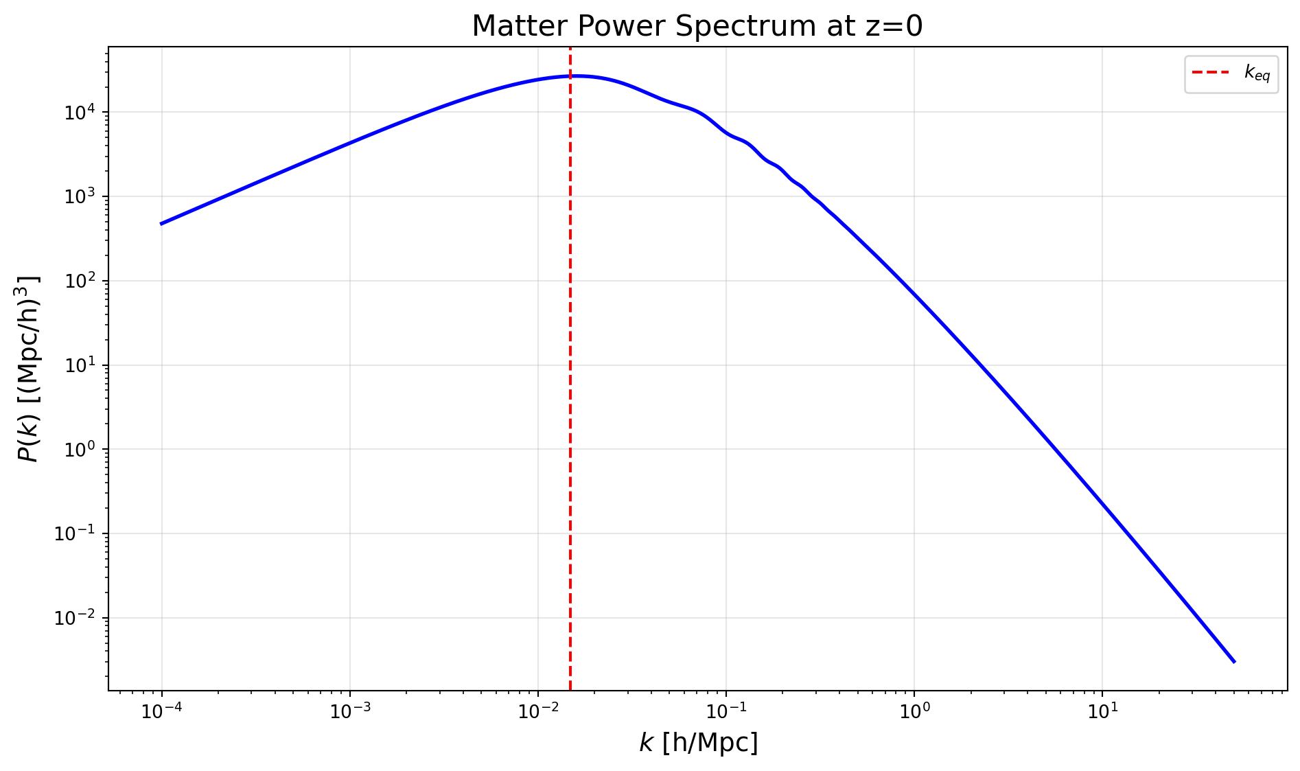
With this in hand, we can easily explore how the matter power spectrum changes as we vary cosmological parameters. We’ll do some simple examples here, paralleling the discussion in lecture.
The simplest variation is to change the amplitude of the primordial power spectrum, \(A_s\). This will simply scale the matter power spectrum up or down without changing its shape.
# Define a set of A_s values to explore
A_s_values = [1.5e-9, 2.1e-9, 3.0e-9]
colors = ['blue', 'black', 'red']
labels = [r'$A_s = 1.5 \times 10^{-9}$',
          r'$A_s = 2.1 \times 10^{-9}$ (fiducial)',
          r'$A_s = 3.0 \times 10^{-9}$']

plt.figure(figsize=(10, 6))

for A_s, color, label in zip(A_s_values, colors, labels):
    # Create CLASS instance
    cosmo = Class()

    # Set cosmological parameters
    cosmo.set({
        'output': 'mPk',
        'h': 0.7,
        'omega_b': 0.02237,
        'omega_cdm': 0.1200,
        'A_s': A_s,              # Vary this parameter
        'n_s': 0.9649,
        'P_k_max_h/Mpc': 50.0,
        'z_max_pk': 0.0
    })

    # Compute
    cosmo.compute()

    # Get power spectrum
    h = cosmo.h
    k_h_values = np.logspace(-4, np.log10(50.0), 1000)
    pk_values = np.array([cosmo.pk(k*h, 0.0)*h**3 for k in k_h_values])

    # Plot
    plt.loglog(k_h_values, pk_values, color=color, linewidth=2, label=label)

    # Clean up
    cosmo.struct_cleanup()

plt.xlabel(r'$k$ [h/Mpc]', fontsize=14)
plt.ylabel(r'$P(k)$ [(Mpc/h)$^3$]', fontsize=14)
plt.title(r'Matter Power Spectrum: Varying $A_s$', fontsize=16)
plt.legend(fontsize=12)
plt.grid(True, alpha=0.3)
plt.tight_layout()
plt.show()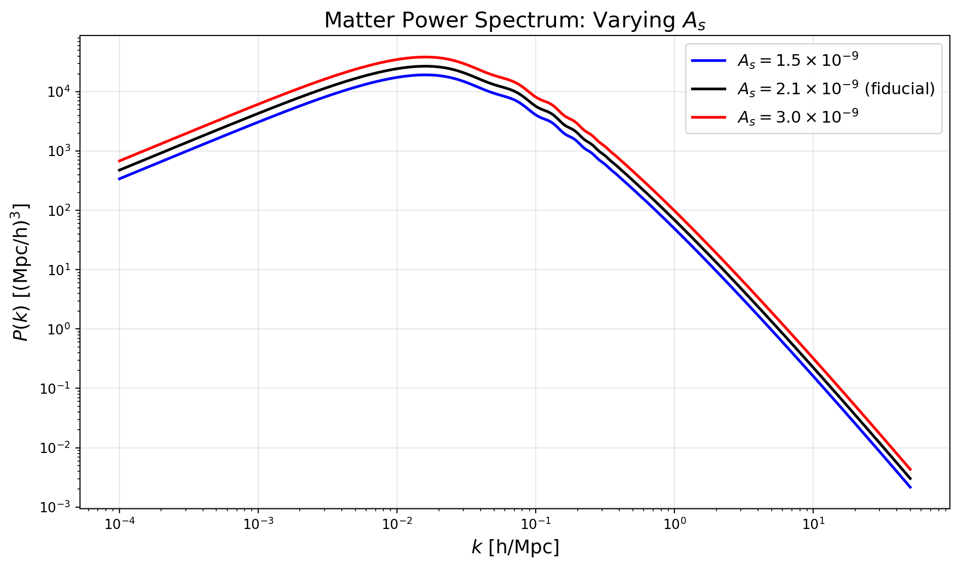
Changing the spectral index will change the overall tilt of the power spectrum on both sides of the turnover.
We also plot our expectations for the slope in the two regimes for the reference model :
# Define a set of n_s values to explore
# Using different A_s values to offset curves for clarity
fiducial_n_s = 1.0
n_s_values = [fiducial_n_s, 0.90, 1.10]
A_s_values = [2e-9, 0.5e-9, 8.0e-9]  # Artificially different to separate curves
colors = ['black', 'blue', 'red']
labels = [rf'$n_s = {n_s:.2f}$' + (' (fiducial)' if n_s == fiducial_n_s else '')
          for n_s in n_s_values]

plt.figure(figsize=(10, 6))

# First plot the power spectra
for n_s, A_s, color, label in zip(n_s_values, A_s_values, colors, labels):
    # Create CLASS instance
    cosmo = Class()

    # Set cosmological parameters
    cosmo.set({
        'output': 'mPk',
        'h': 0.7,
        'omega_b': 0.02237,
        'omega_cdm': 0.1200,
        'A_s': A_s,              # Artificially varied for clarity
        'n_s': n_s,              # Vary this parameter
        'P_k_max_h/Mpc': 50.0,
        'z_max_pk': 0.0
    })

    # Compute
    cosmo.compute()

    # Get power spectrum
    h = cosmo.h
    k_h_values = np.logspace(-4, np.log10(50.0), 1000)
    pk_values = np.array([cosmo.pk(k*h, 0.0)*h**3 for k in k_h_values])

    # Plot
    plt.loglog(k_h_values, pk_values, color=color, linewidth=2, label=label)

    # For the fiducial model, also plot the expected slopes
    if n_s == fiducial_n_s:
        k_eq = cosmo.k_eq() / h  # Convert to h/Mpc

        # Plot expected slope for k << k_eq: P(k) ~ k^n_s
        k_low = np.logspace(-4, np.log10(k_eq), 50)
        # Normalize at k = 0.001 h/Mpc
        k_norm = 0.001
        idx_norm = np.argmin(np.abs(k_h_values - k_norm))
        pk_norm = pk_values[idx_norm]
        pk_low_expected = pk_norm * (k_low / k_norm)**n_s
        plt.loglog(k_low, pk_low_expected, 'k--', linewidth=1.5,
                   label=r'$\propto k^{n_s}$', alpha=0.6)

        # Plot expected slope for k >> k_eq: P(k) ~ k^(n_s - 4)
        k_high = np.logspace(np.log10(k_eq) + 0.5, np.log10(50.0), 50)
        # Normalize at k = 5.0 h/Mpc
        k_norm_high = 5.0
        idx_norm_high = np.argmin(np.abs(k_h_values - k_norm_high))
        pk_norm_high = pk_values[idx_norm_high]
        pk_high_expected = pk_norm_high * (k_high / k_norm_high)**(n_s - 4)
        plt.loglog(k_high, pk_high_expected, 'k:', linewidth=1.5,
                   label=r'$\propto k^{n_s - 4}$', alpha=0.6)

        # Add a second guide: k^(n_s-4) ln(k/k_eq)^2, anchored at k=5 h/Mpc
        k_anchor = 5.0
        log_anchor = np.log(k_anchor / k_eq)**2
        pk_anchor_plaw = pk_norm_high * (k_anchor / k_norm_high)**(n_s - 4)
        pk_high_log_expected = (pk_anchor_plaw
                    * (k_high / k_anchor)**(n_s - 4)
                    * (np.log(k_high / k_eq)**2 / log_anchor))
        plt.loglog(k_high, pk_high_log_expected, 'k-.', linewidth=1.5,
               label=r'$\propto k^{n_s - 4}\,\ln^2(k/k_{eq})$', alpha=0.6)

        # Mark k_eq
        plt.axvline(k_eq, color='gray', linestyle='--', linewidth=1, alpha=0.5)
        plt.text(k_eq*1.2, plt.ylim()[0] * 1.5, r'$k_{eq}$',
                ha='center', fontsize=10, color='gray')

    # Clean up
    cosmo.struct_cleanup()

plt.xlabel(r'$k$ [h/Mpc]', fontsize=14)
plt.ylabel(r'$P(k)$ [(Mpc/h)$^3$]', fontsize=14)
plt.title(r'Matter Power Spectrum: Varying $n_s$', fontsize=16)
plt.text(0.02, 0.02, '(Amplitudes artificially offset for clarity)',
         transform=plt.gca().transAxes, fontsize=10, style='italic', alpha=0.7)
plt.legend(fontsize=11, loc='upper left')
plt.grid(True, alpha=0.3)
plt.tight_layout()
plt.show()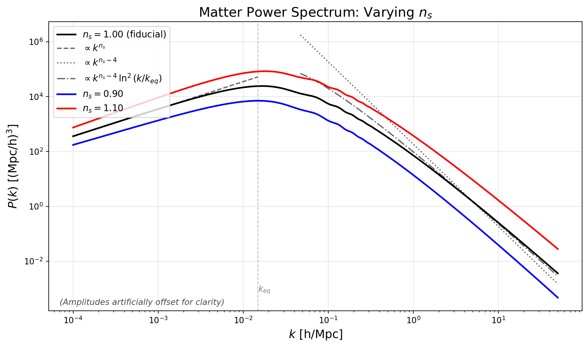
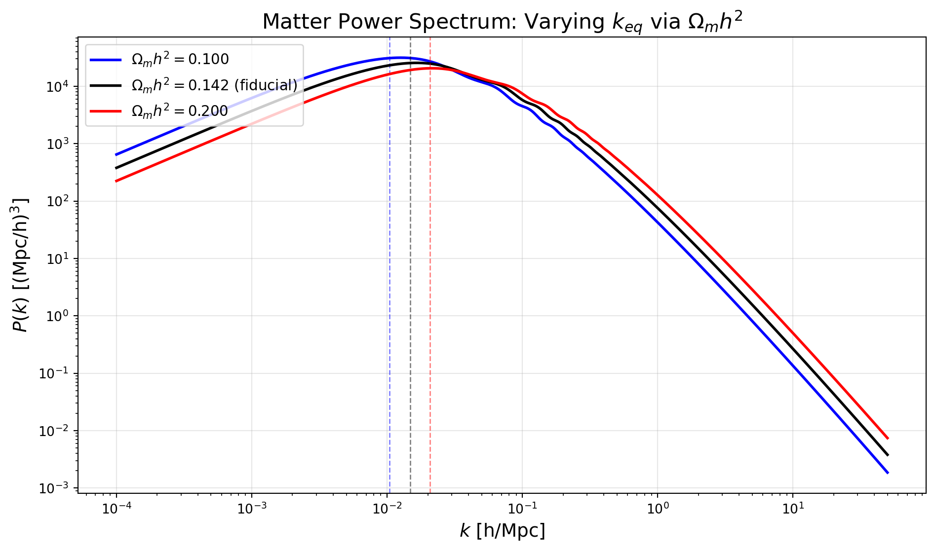
Let’s now consider varying the matter-radiation equality scale \(k_{eq}\) and therefore shift the location of the turnover in the power spectrum. This is determined by the matter density \(\Omega_m h^2\) and the radiation density (which is fixed by the CMB temperature).
Recall from lecture that the turnover scale is given by \[ k_{eq} = H_0 \sqrt{\frac{2 \Omega_m^2}{\Omega_r}} \] where \(\Omega_r\) is the radiation density parameter.
Physically, the temperature of the CMB is very well measured, so the photon density is fixed. We could varying the number of relativistic species (e.g. neutrinos) to change the radiation density, but for simplicity we will just vary \(\Omega_m h^2\) to shift \(k_{eq}\). We will do so, but keep the ratio of baryons to CDM fixed to avoid changing the shape of the power spectrum in other ways.
# Fiducial densities and baryon fraction
omega_b_fid = 0.02237
omega_cdm_fid = 0.1200
omega_mh2_fid = omega_b_fid + omega_cdm_fid
f_b = omega_b_fid / omega_mh2_fid

# Vary Omega_m h^2 while keeping baryon fraction fixed
omega_mh2_values = [0.10, omega_mh2_fid, 0.20]
colors = ['blue', 'black', 'red']
labels = [rf'$\Omega_m h^2 = {val:.3f}$' + (' (fiducial)' if val == omega_mh2_fid else '')
          for val in omega_mh2_values]

plt.figure(figsize=(10, 6))

for omega_mh2, color, label in zip(omega_mh2_values, colors, labels):
    omega_b = f_b * omega_mh2
    omega_cdm = (1.0 - f_b) * omega_mh2

    # Create CLASS instance
    cosmo = Class()

    # Set cosmological parameters
    cosmo.set({
        'output': 'mPk',
        'h': 0.7,
        'omega_b': omega_b,
        'omega_cdm': omega_cdm,
        'A_s': 2.1e-9,
        'n_s': 1.0,
        'P_k_max_h/Mpc': 50.0,
        'z_max_pk': 0.0
    })

    # Compute
    cosmo.compute()

    # Get power spectrum
    h = cosmo.h
    k_h_values = np.logspace(-4, np.log10(50.0), 1000)
    pk_values = np.array([cosmo.pk(k*h, 0.0)*h**3 for k in k_h_values])

    # Plot
    plt.loglog(k_h_values, pk_values, color=color, linewidth=2, label=label)

    # Mark k_eq for each curve
    k_eq = cosmo.k_eq() / h
    plt.axvline(k_eq, color=color, linestyle='--', linewidth=1, alpha=0.5)

    # Clean up
    cosmo.struct_cleanup()

plt.xlabel(r'$k$ [h/Mpc]', fontsize=14)
plt.ylabel(r'$P(k)$ [(Mpc/h)$^3$]', fontsize=14)
plt.title(r'Matter Power Spectrum: Varying $k_{eq}$ via $\Omega_m h^2$', fontsize=16)
plt.legend(fontsize=11, loc='upper left')
plt.grid(True, alpha=0.3)
plt.tight_layout()
plt.show()