# Cosmological Simulations III: Analysis
## Introduction
In the previous lecture, we built a Particle-Mesh (PM) $N$-body code from
scratch — implementing CIC mass assignment, an FFT-based Poisson solver, and
a symplectic KDK leapfrog integrator. We tested it against the Zel'dovich
approximation and ran a $128^3$ cosmological simulation to see the cosmic web
emerge.
In this lecture, we push the resolution to $256^3$ and analyze the simulation
output in detail: density fields, power spectra, growth factors, redshift-space
distortions, and RSD multipoles. Along the way, we will connect the simulation
results back to the linear theory we developed earlier in the course.
## Setup
### PM Code
All the PM functions from the previous lecture are collected below. This is
the same code — `cic_deposit`, `cic_interp`, `make_green_function`,
`pm_force`, `kdk_step`, `run_simulation`, and supporting utilities — copied
verbatim so that this notebook is self-contained.
```{python}
#| code-fold: true
#| code-summary: "PM code from Lecture 20"
import jax
import jax.numpy as jnp
from jax import jit
from functools import partial

def hubble(a):
    """H(a) / H_0 for Einstein-de Sitter."""
    return a**(-1.5)

def drift_factor(a1, a2):
    """D(a1, a2) = 2 (1/sqrt(a1) - 1/sqrt(a2)) for EdS (H_0 = 1)."""
    return 2.0 * (1.0 / jnp.sqrt(a1) - 1.0 / jnp.sqrt(a2))

def kick_factor(a1, a2):
    """K(a1, a2) = (2/3) (a2^{3/2} - a1^{3/2}) for EdS (H_0 = 1)."""
    return (2.0 / 3.0) * (a2**1.5 - a1**1.5)

def cic_deposit(pos, Ng, L):
    """
    CIC mass assignment: deposit unit-mass particles onto an Ng^3 grid.

    Parameters
    ----------
    pos : array, shape (N, 3)
        Particle positions in [0, L).
    Ng : int
        Grid size per dimension.
    L : float
        Box size.

    Returns
    -------
    rho : array, shape (Ng, Ng, Ng)
        Density field (particle count per cell).
    """
    h = L / Ng

    # Wrap positions into [0, L)
    pos = pos % L

    # Grid index of lower-left corner and fractional offset
    cell = (pos / h - 0.5)          # shifted so grid points are at centers
    idx = jnp.floor(cell).astype(int)
    dx = cell - idx                 # fractional distance, in [0, 1)

    # CIC weights: 1 - dx for the lower grid point, dx for the upper
    wx = jnp.stack([1.0 - dx, dx], axis=-1)  # shape (N, 3, 2)

    # Build the 2^3 = 8 contributions
    rho = jnp.zeros((Ng, Ng, Ng))
    for ii in range(2):
        for jj in range(2):
            for kk in range(2):
                weight = wx[:, 0, ii] * wx[:, 1, jj] * wx[:, 2, kk]
                ix = (idx[:, 0] + ii) % Ng
                iy = (idx[:, 1] + jj) % Ng
                iz = (idx[:, 2] + kk) % Ng
                rho = rho.at[ix, iy, iz].add(weight)

    return rho

def cic_interp(field, pos, Ng, L):
    """
    CIC interpolation: read a grid field at particle positions.

    Parameters
    ----------
    field : array, shape (Ng, Ng, Ng)
        Field defined on the grid.
    pos : array, shape (N, 3)
        Particle positions in [0, L).

    Returns
    -------
    values : array, shape (N,)
        Interpolated field values at particle positions.
    """
    h = L / Ng
    pos = pos % L

    cell = (pos / h - 0.5)
    idx = jnp.floor(cell).astype(int)
    dx = cell - idx

    wx = jnp.stack([1.0 - dx, dx], axis=-1)

    values = jnp.zeros(pos.shape[0])
    for ii in range(2):
        for jj in range(2):
            for kk in range(2):
                weight = wx[:, 0, ii] * wx[:, 1, jj] * wx[:, 2, kk]
                ix = (idx[:, 0] + ii) % Ng
                iy = (idx[:, 1] + jj) % Ng
                iz = (idx[:, 2] + kk) % Ng
                values = values + weight * field[ix, iy, iz]

    return values

def make_green_function(Ng, L):
    """
    Precompute the Green's function for the PM force calculation.

    Returns the gradient of the inverse Laplacian in Fourier space:
    G_i(k) = D_i(k) / L(k), with discrete operators.

    Returns
    -------
    green_x, green_y, green_z : arrays, shape (Ng, Ng, Ng)
        Fourier-space Green's function for each force component.
    """
    h = L / Ng

    # Wavenumber indices
    k = jnp.fft.fftfreq(Ng, d=1.0/Ng)  # integer wavenumber indices 0..Ng/2..-1
    kx, ky, kz = jnp.meshgrid(k, k, k, indexing='ij')

    # Discrete Laplacian: -sum_i (4/h^2) sin^2(pi k_i / Ng)
    laplacian = -(4.0 / h**2) * (
        jnp.sin(jnp.pi * kx / Ng)**2 +
        jnp.sin(jnp.pi * ky / Ng)**2 +
        jnp.sin(jnp.pi * kz / Ng)**2
    )

    # Avoid division by zero at k=0
    laplacian = laplacian.at[0, 0, 0].set(1.0)

    # Discrete gradient: (i/h) sin(2 pi k_i / Ng)
    grad_x = 1j / h * jnp.sin(2.0 * jnp.pi * kx / Ng)
    grad_y = 1j / h * jnp.sin(2.0 * jnp.pi * ky / Ng)
    grad_z = 1j / h * jnp.sin(2.0 * jnp.pi * kz / Ng)

    # Green's function: G_i = D_i / L
    green_x = grad_x / laplacian
    green_y = grad_y / laplacian
    green_z = grad_z / laplacian

    # Zero the k=0 mode (no mean force)
    green_x = green_x.at[0, 0, 0].set(0.0)
    green_y = green_y.at[0, 0, 0].set(0.0)
    green_z = green_z.at[0, 0, 0].set(0.0)

    return green_x, green_y, green_z

def pm_force(pos, a, green_x, green_y, green_z, Ng, L, Omega_m):
    """
    Compute -grad(Phi) at each particle position via the PM method.

    The kick step is: dp = -grad(Phi) * K(a1, a2).
    This function returns -grad(Phi), including the Poisson prefactor
    (3/2) Omega_m / a.  The caller multiplies by the kick factor.

    Parameters
    ----------
    pos : array, shape (N, 3)
        Particle positions in [0, L).
    a : float
        Scale factor.
    green_x, green_y, green_z : arrays
        Precomputed Green's functions.
    Ng : int
        Grid size per dimension.
    L : float
        Box size.
    Omega_m : float
        Matter density parameter.

    Returns
    -------
    force : array, shape (N, 3)
        -grad(Phi) at each particle position.
    """
    # 1. CIC deposit
    rho = cic_deposit(pos, Ng, L)

    # 2. Overdensity: delta = rho / rho_bar - 1, where rho_bar = N / Ng^3
    rho_bar = pos.shape[0] / Ng**3
    delta = rho / rho_bar - 1.0

    # 3. Forward FFT
    delta_hat = jnp.fft.fftn(delta)

    # 4. Poisson prefactor: (3/2) Omega_m / a  (in H_0=1 units)
    prefactor = 1.5 * Omega_m / a

    # 5. Force in Fourier space: -prefactor * G_i * delta_hat
    fx_hat = -prefactor * green_x * delta_hat
    fy_hat = -prefactor * green_y * delta_hat
    fz_hat = -prefactor * green_z * delta_hat

    # 6. Inverse FFT (force fields are real)
    fx = jnp.fft.ifftn(fx_hat).real
    fy = jnp.fft.ifftn(fy_hat).real
    fz = jnp.fft.ifftn(fz_hat).real

    # 7. CIC interpolate to particle positions
    ax = cic_interp(fx, pos, Ng, L)
    ay = cic_interp(fy, pos, Ng, L)
    az = cic_interp(fz, pos, Ng, L)

    return jnp.stack([ax, ay, az], axis=-1)

def kdk_step(pos, mom, a_start, a_end, green_x, green_y, green_z,
             Ng, L, Omega_m):
    """
    One KDK leapfrog step from a_start to a_end.

    Parameters
    ----------
    pos : array, shape (N, 3)
        Comoving positions.
    mom : array, shape (N, 3)
        Conjugate momenta (p = m a^2 dx/dt; m=1 here).
    a_start, a_end : float
        Scale factor at start and end of step.
    green_x, green_y, green_z : arrays
        Precomputed Green's functions.

    Returns
    -------
    pos_new, mom_new : arrays
        Updated positions and momenta.
    """
    a_mid = 0.5 * (a_start + a_end)

    # Half kick
    K1 = kick_factor(a_start, a_mid)
    force = pm_force(pos, a_start, green_x, green_y, green_z, Ng, L, Omega_m)
    mom = mom + force * K1

    # Full drift
    D = drift_factor(a_start, a_end)
    pos = pos + mom * D
    pos = pos % L   # periodic wrapping

    # Half kick
    K2 = kick_factor(a_mid, a_end)
    force = pm_force(pos, a_end, green_x, green_y, green_z, Ng, L, Omega_m)
    mom = mom + force * K2

    return pos, mom

@partial(jit, static_argnums=(4, 8))
def run_simulation(pos_init, mom_init, a_start, a_end, n_steps,
                   green_x, green_y, green_z, Ng, L, Omega_m):
    """
    Run PM N-body simulation from a_start to a_end.

    Uses equally-spaced steps in ln(a), and avoids redundant force
    evaluations by merging half-kicks. The entire simulation is
    JIT-compiled using jax.lax.fori_loop.

    Parameters
    ----------
    n_steps : int (static)
        Number of timesteps.
    Ng : int (static)
        Grid size per dimension.

    Returns
    -------
    pos, mom : arrays
        Final positions and momenta.
    """
    # Steps equally spaced in ln(a)
    a_values = jnp.exp(jnp.linspace(jnp.log(a_start), jnp.log(a_end), n_steps + 1))
    a_mid = 0.5 * (a_values[:-1] + a_values[1:])  # midpoints, length n_steps

    # Precompute all drift factors: D(a_n, a_{n+1})
    D_arr = jax.vmap(drift_factor)(a_values[:-1], a_values[1:])

    # Precompute all kick factors for the merged scheme.
    # Step i kicks from a_mid[i] to a_mid[i+1],
    # except the last step kicks from a_mid[-1] to a_values[-1].
    kick_ends = jnp.concatenate([a_mid[1:], a_values[-1:]])
    K_arr = jax.vmap(kick_factor)(a_mid, kick_ends)

    # Initial half-kick
    K_init = kick_factor(a_values[0], a_mid[0])
    force = pm_force(pos_init, a_values[0], green_x, green_y, green_z, Ng, L, Omega_m)
    mom_init = mom_init + force * K_init

    def body(i, carry):
        pos, mom = carry
        # Full drift
        pos = pos + mom * D_arr[i]
        pos = pos % L
        # Force at a_{n+1}, then merged kick
        force = pm_force(pos, a_values[i + 1], green_x, green_y, green_z, Ng, L, Omega_m)
        mom = mom + force * K_arr[i]
        return pos, mom

    pos, mom = jax.lax.fori_loop(0, n_steps, body, (pos_init, mom_init))
    return pos, mom

def make_uniform_grid(Np, L):
    """Create a uniform grid of Np^3 particles in a box of side L."""
    x = jnp.linspace(0, L, Np, endpoint=False) + L / (2 * Np)
    grid = jnp.meshgrid(x, x, x, indexing='ij')
    pos = jnp.stack([g.ravel() for g in grid], axis=-1)
    return pos
```
### Imports and Parameters
```{python}
import numpy as np
import matplotlib.pyplot as plt
from scipy.interpolate import interp1d
import time
```
```{python}
# Simulation parameters
Ng = 256             # grid cells per dimension
Np = 256             # particles per dimension (= Ng for this run)
L = 500.0            # box size in Mpc/h
Omega_m = 1.0        # Einstein-de Sitter
z_init = 49.0        # starting redshift
a_init = 1.0 / (1.0 + z_init)
a_final = 1.0        # z = 0
n_steps = 100        # number of timesteps

print(f"Grid: {Ng}^3 = {Ng**3:,} cells")
print(f"Particles: {Np}^3 = {Np**3:,}")
print(f"Box: L = {L} Mpc/h")
print(f"Redshift: z = {z_init} → 0  (a = {a_init:.4f} → {a_final})")
print(f"Steps: {n_steps} (log-spaced in a)")
```
::: {.callout-note}
## Choice of Timestep Count
We use 100 steps for this simulation. The KDK leapfrog is second-order, and
with steps equally spaced in $\ln a$ the resolution is finest at early times
when structures are forming most rapidly. For our EdS cosmology and the
observables we measure in this lecture (power spectra, growth factors, RSD
multipoles), we have verified that 100 steps gives sub-percent agreement
with 200 steps across all scales.
This should not be taken as a general rule. The required number of steps
depends on the cosmology, the box size, the force resolution, and the
observables of interest. Any production simulation requires its own
convergence tests — the right approach is to run at two different step
counts and verify that your results are insensitive to the choice.
:::
### Power Spectrum from CLASS
We use CLASS to compute the linear power spectrum $P(k)$ at $z = 0$, which
serves as input for the initial conditions and as a reference for comparison
later.
```{python}
from classy import Class

cosmo = Class()
cosmo.set({
    'output': 'mPk',
    'h': 0.7,
    'omega_b': 0.02237,
    'omega_cdm': 0.1200,
    'A_s': 2.1e-9,
    'n_s': 0.9649,
    'P_k_max_h/Mpc': 50.0,
    'z_max_pk': 100.0
})
cosmo.compute()

h_class = cosmo.h()
print(f"CLASS cosmology: Omega_m = {cosmo.Omega_m():.4f}, "
      f"h = {h_class:.3f}, sigma8 = {cosmo.sigma8():.4f}")

# Build the P(k) interpolator at z=0
k_arr = np.logspace(-4, np.log10(50.0), 2000)  # k in h/Mpc
pk_arr = np.array([cosmo.pk(k * h_class, 0.0) * h_class**3
                   for k in k_arr])  # P(k, z=0) in (Mpc/h)^3
cosmo.struct_cleanup()

log_pk_interp = interp1d(np.log(k_arr), np.log(pk_arr),
                         kind='cubic', fill_value=-100.0,
                         bounds_error=False)

def pk_of_k(k):
    """P(k) in (Mpc/h)^3, k in h/Mpc."""
    return np.exp(log_pk_interp(np.log(k)))

print(f"Box: L = {L} Mpc/h")
print(f"Fundamental mode: k_f = {2*np.pi/L:.4f} h/Mpc")
print(f"Nyquist: k_Ny = {np.pi*Ng/L:.2f} h/Mpc")
```
### Generating Initial Conditions
We generate Gaussian random initial conditions using the Zel'dovich
approximation, exactly as in Lecture 20. The procedure: draw a white noise
field, color it with $\sqrt{P(k)}$ to create the $z = 0$ density field
$\delta_0$, compute the displacement field $\boldsymbol{\Psi}$ via
$\Psi_i(\mathbf{k}) = -i k_i / k^2 \, \hat{\delta}_0(\mathbf{k})$, then
displace particles from a uniform grid by $D_+(a_\text{init}) \,
\boldsymbol{\Psi}$.
```{python}
def make_cosmo_ic(Np, Ng, L, pk_func, a_init, seed=42):
    """
    Generate cosmological Zel'dovich ICs from a power spectrum.

    Returns positions, momenta, the Lagrangian grid, and the z=0
    linear density field (for later comparison with the simulation).
    """
    h = L / Ng
    V = L**3

    # Wavenumber grid
    kfreq = 2 * np.pi * np.fft.fftfreq(Ng, d=h)
    kx, ky, kz = np.meshgrid(kfreq, kfreq, kfreq, indexing='ij')
    kmag = np.sqrt(kx**2 + ky**2 + kz**2)
    kmag[0, 0, 0] = 1.0  # avoid division by zero

    # Power spectrum on the grid
    pk_grid = pk_func(kmag)
    pk_grid[0, 0, 0] = 0.0

    # Gaussian random field: color white noise with sqrt(P(k))
    rng = np.random.default_rng(seed)
    white_noise = rng.standard_normal((Ng, Ng, Ng))
    noise_hat = np.fft.fftn(white_noise)

    amplitude = Ng**1.5 * np.sqrt(pk_grid / V)
    delta_hat = amplitude * noise_hat
    delta_hat[0, 0, 0] = 0.0

    # Displacement field: Psi_i(k) = -i k_i / k^2 * delta_hat(k)
    inv_k2 = 1.0 / (kmag**2)
    inv_k2[0, 0, 0] = 0.0

    psi_hat_x = -1j * kx * inv_k2 * delta_hat
    psi_hat_y = -1j * ky * inv_k2 * delta_hat
    psi_hat_z = -1j * kz * inv_k2 * delta_hat

    psi_x = np.fft.ifftn(psi_hat_x).real
    psi_y = np.fft.ifftn(psi_hat_y).real
    psi_z = np.fft.ifftn(psi_hat_z).real

    # Lagrangian grid
    q = make_uniform_grid(Np, L)
    q_np = np.array(q)

    # Interpolate displacement to particle positions (Np = Ng: direct indexing)
    idx = np.round(q_np / h - 0.5).astype(int) % Ng
    psi_at_q = np.stack([
        psi_x[idx[:, 0], idx[:, 1], idx[:, 2]],
        psi_y[idx[:, 0], idx[:, 1], idx[:, 2]],
        psi_z[idx[:, 0], idx[:, 1], idx[:, 2]],
    ], axis=-1)

    # Zel'dovich: x = q + D_+(a) * Psi, p = a^{3/2} * Psi  (EdS)
    pos = jnp.array((q_np + a_init * psi_at_q) % L)
    mom = jnp.array(a_init**1.5 * psi_at_q)

    # Also return the z=0 linear density field (delta_hat is at z=0)
    delta0 = np.fft.ifftn(delta_hat).real

    return pos, mom, q, delta0

import os
DATA_DIR = os.path.expanduser("~/data/teaching/ASTR6000-SP26")
CACHE_DIR = os.path.join(DATA_DIR, "021-pm-analysis")
os.makedirs(CACHE_DIR, exist_ok=True)
```
### Running the Simulation
We precompute the Green's function, then run the simulation from $z = 49$
to $z = 0$. We also run to several intermediate redshifts ($z = 9, 4, 1$)
so that we can study the growth of structure over time in later sections.
Each run uses a proportional number of timesteps, keeping the step size in
$\ln a$ consistent.
Results (including the initial conditions and the $z = 0$ linear density
field) are cached to disk as separate files so that subsequent renders skip
the simulation entirely, and individual snapshots can be regenerated without
invalidating the rest.
```{python}
# Snapshot redshifts and corresponding scale factors
z_snapshots = [9, 4, 1, 0]
a_snapshots = [1.0 / (1.0 + z) for z in z_snapshots]

# --- Load or generate ICs ---
ic_file = os.path.join(CACHE_DIR, "ic.npz")

if os.path.exists(ic_file):
    print(f"Loading cached ICs from {ic_file}")
    cached_ic = np.load(ic_file)
    pos_ic = jnp.array(cached_ic['pos_ic'])
    mom_ic = jnp.array(cached_ic['mom_ic'])
    delta0_z0 = cached_ic['delta0_z0']
else:
    print("Generating initial conditions...")
    pos_ic, mom_ic, q_grid, delta0_z0 = make_cosmo_ic(
        Np, Ng, L, pk_of_k, a_init, seed=42
    )
    print(f"  rms displacement: {np.std(np.array(pos_ic - q_grid)):.4f} Mpc/h")
    np.savez(ic_file, pos_ic=np.array(pos_ic), mom_ic=np.array(mom_ic),
             delta0_z0=delta0_z0)
    print(f"  Saved to {ic_file}")

print(f"Particles: {pos_ic.shape[0]:,}")

# --- Load or run snapshots ---
snapshots = {}
need_to_run = []

for z_snap, a_snap in zip(z_snapshots, a_snapshots):
    snap_file = os.path.join(CACHE_DIR, f"snap_z{z_snap}.npz")
    if os.path.exists(snap_file):
        cached_snap = np.load(snap_file)
        snapshots[z_snap] = {
            'pos': jnp.array(cached_snap['pos']),
            'mom': jnp.array(cached_snap['mom']),
            'a': a_snap,
        }
        print(f"  z={z_snap}: loaded from cache")
    else:
        need_to_run.append((z_snap, a_snap))

if need_to_run:
    print(f"\nRunning {len(need_to_run)} simulation(s)...")
    green_x, green_y, green_z = make_green_function(Ng, L)
    log_range_total = np.log(a_final) - np.log(a_init)
    t_total = 0.0

    for z_snap, a_snap in need_to_run:
        log_range = np.log(a_snap) - np.log(a_init)
        n_snap = max(10, int(round(n_steps * log_range / log_range_total)))

        print(f"  z = {z_snap} (a = {a_snap:.3f}), {n_snap} steps...",
              end=" ", flush=True)
        t0 = time.perf_counter()
        pos_f, mom_f = run_simulation(
            pos_ic, mom_ic, a_init, a_snap, n_snap,
            green_x, green_y, green_z, Ng, L, Omega_m
        )
        pos_f.block_until_ready()
        mom_f.block_until_ready()
        dt = time.perf_counter() - t0
        t_total += dt
        print(f"{dt:.1f}s")

        snapshots[z_snap] = {'pos': pos_f, 'mom': mom_f, 'a': a_snap}

        snap_file = os.path.join(CACHE_DIR, f"snap_z{z_snap}.npz")
        np.savez(snap_file, pos=np.array(pos_f), mom=np.array(mom_f))

    print(f"\nTotal simulation time: {t_total:.1f}s")
else:
    print("\nAll snapshots loaded from cache.")
```
::: {.callout-note}
## Compilation Overhead
The first simulation triggers JAX's JIT compilation — tracing the entire
computation graph and compiling it to optimized machine code via XLA. This
is a one-time cost; subsequent runs with the same `n_steps` and `Ng` reuse
the cached compilation and execute much faster. Runs with different step
counts trigger recompilation (since `n_steps` is a static argument), but
each compilation is reused for any future call with the same count.
:::
### Analysis Utilities
We will repeatedly need to deposit particles onto the grid and measure power
spectra throughout this lecture. Here we set up JIT-compiled and vectorized
versions of these operations.
```{python}
#| code-fold: true
#| code-summary: "Analysis utilities: CIC deposit (JIT) and power spectrum measurement"
# JIT-compiled CIC deposit for standalone use (Ng is static)
cic_deposit_jit = jax.jit(cic_deposit, static_argnums=(1,))

def deposit_to_delta(pos, Ng, L):
    """Deposit particles and return the overdensity field delta as a numpy array."""
    rho = cic_deposit_jit(pos, Ng, L)
    rho_bar = pos.shape[0] / Ng**3
    return np.array(rho / rho_bar - 1.0)

def make_k_grid(Ng, L, n_mu_bins=10):
    """
    Precompute wavenumber grid, bin assignments, and mu for P(k, mu) measurement.

    Returns a dict with:
        kmag       : (Ng, Ng, Ng) array of |k|
        mu         : (Ng, Ng, Ng) array of k_z / |k| (LOS along z)
        ik         : (Ng^3,) int array of radial k-bin index (flattened)
        imu        : (Ng^3,) int array of |mu| bin index (flattened)
        k_centers  : (n_k_bins,) radial bin centers
        mu_centers : (n_mu_bins,) |mu| bin centers
        n_k_bins   : number of radial bins
        n_mu_bins  : number of |mu| bins
        norm       : h^6 / V prefactor for P(k) normalization
    """
    h = L / Ng
    V = L**3
    kfreq = 2 * jnp.pi * jnp.fft.fftfreq(Ng, d=h)
    kx, ky, kz = jnp.meshgrid(kfreq, kfreq, kfreq, indexing='ij')
    kmag = jnp.sqrt(kx**2 + ky**2 + kz**2)

    # mu = k_z / |k| (line of sight along z-axis)
    kmag_safe = jnp.where(kmag == 0, 1.0, kmag)
    mu = kz / kmag_safe
    mu = jnp.where(kmag == 0, 0.0, mu)

    # Radial k bins: k_fund/2 to k_Nyquist, spaced by k_fund
    k_fund = 2 * jnp.pi / L
    k_nyq = jnp.pi * Ng / L
    k_edges = jnp.arange(k_fund / 2, k_nyq + k_fund, k_fund)
    n_k_bins = len(k_edges) - 1
    k_centers = 0.5 * (k_edges[:-1] + k_edges[1:])

    # |mu| bins: 0 to 1 (symmetric in mu, so bin |mu|)
    mu_edges = jnp.linspace(0, 1, n_mu_bins + 1)
    mu_centers = 0.5 * (mu_edges[:-1] + mu_edges[1:])

    # Bin assignments (flattened)
    ik = jnp.digitize(kmag.ravel(), k_edges) - 1
    imu = jnp.digitize(jnp.abs(mu).ravel(), mu_edges) - 1
    imu = jnp.clip(imu, 0, n_mu_bins - 1)  # |mu|=1 edge case

    # Effective k per bin: mean |k| of modes in each bin
    kmag_flat = kmag.ravel()
    k_sum = jnp.zeros(n_k_bins).at[ik].add(kmag_flat, mode='drop')
    k_count = jnp.zeros(n_k_bins).at[ik].add(jnp.ones_like(kmag_flat), mode='drop')
    k_eff = jnp.where(k_count > 0, k_sum / k_count, k_centers)

    return {
        'ik': ik, 'imu': imu,
        'k_eff': k_eff, 'k_centers': k_centers, 'mu_centers': mu_centers,
        'k_edges': k_edges, 'mu_edges': mu_edges,
        'n_k_bins': n_k_bins, 'n_mu_bins': n_mu_bins,
        'norm': h**6 / V,
    }

@partial(jax.jit, static_argnums=(2,))
def _bin_power(power_flat, ik, n_k):
    """Scatter-add power into radial k-bins."""
    # mode='drop' silently ignores out-of-range indices (k=0, k>k_Ny)
    pk_sum = jnp.zeros(n_k).at[ik].add(power_flat, mode='drop')
    counts = jnp.zeros(n_k).at[ik].add(jnp.ones_like(power_flat), mode='drop')
    pk = jnp.where(counts > 0, pk_sum / counts, 0.0)
    return pk, counts

def measure_pk(delta, kgrid):
    """
    Measure the isotropic power spectrum P(k) from a 3D density field.

    Uses the DFT convention from Lecture 20:
        delta_hat_continuous(k) = h^3 * delta_hat_DFT(k)
        P(k) = (1/V) * |delta_hat_continuous(k)|^2

    Parameters
    ----------
    delta : array, shape (Ng, Ng, Ng)
        Overdensity field.
    kgrid : dict
        Output of make_k_grid.

    Returns
    -------
    k_centers : array — bin centers in h/Mpc.
    pk : array — power spectrum in (Mpc/h)^3.
    counts : array — number of modes per bin.
    """
    delta_hat = jnp.fft.fftn(jnp.asarray(delta))
    power_flat = jnp.abs(delta_hat).ravel()**2 * kgrid['norm']
    pk, counts = _bin_power(power_flat, kgrid['ik'], kgrid['n_k_bins'])
    return kgrid['k_eff'], pk, counts

# Precompute the k-grid for this box (used by all P(k) measurements)
kgrid = make_k_grid(Ng, L)
```
## Linear vs Nonlinear Density Fields
Our simulation evolved $256^3$ particles under full nonlinear gravity from
$z = 49$ to $z = 0$. How does the result compare to what linear theory
predicts?
The initial conditions were generated from the $z = 0$ linear density field
$\delta_0(\mathbf{x})$, scaled back to $z = 49$ by multiplying by
$D_+(a_\text{init}) = a_\text{init}$ (EdS). To get the linear prediction at
$z = 0$, we simply take $\delta_0$ — since $D_+(a = 1) = 1$ in our
normalization. For the nonlinear field, we deposit the simulation particles
at $z = 0$ onto the grid using CIC.
We use $\operatorname{arcsinh}(\delta/2)$ as the color mapping for all density
field plots. Unlike $\log_{10}(1 + \delta)$, this handles voids ($\delta < 0$)
smoothly and behaves like $\log(\delta)$ at high density.
```{python}
def arcsinh_scale(delta):
    """Color scaling for density fields: arcsinh(delta/2)."""
    return np.arcsinh(np.array(delta) / 2.0)
```
```{python}
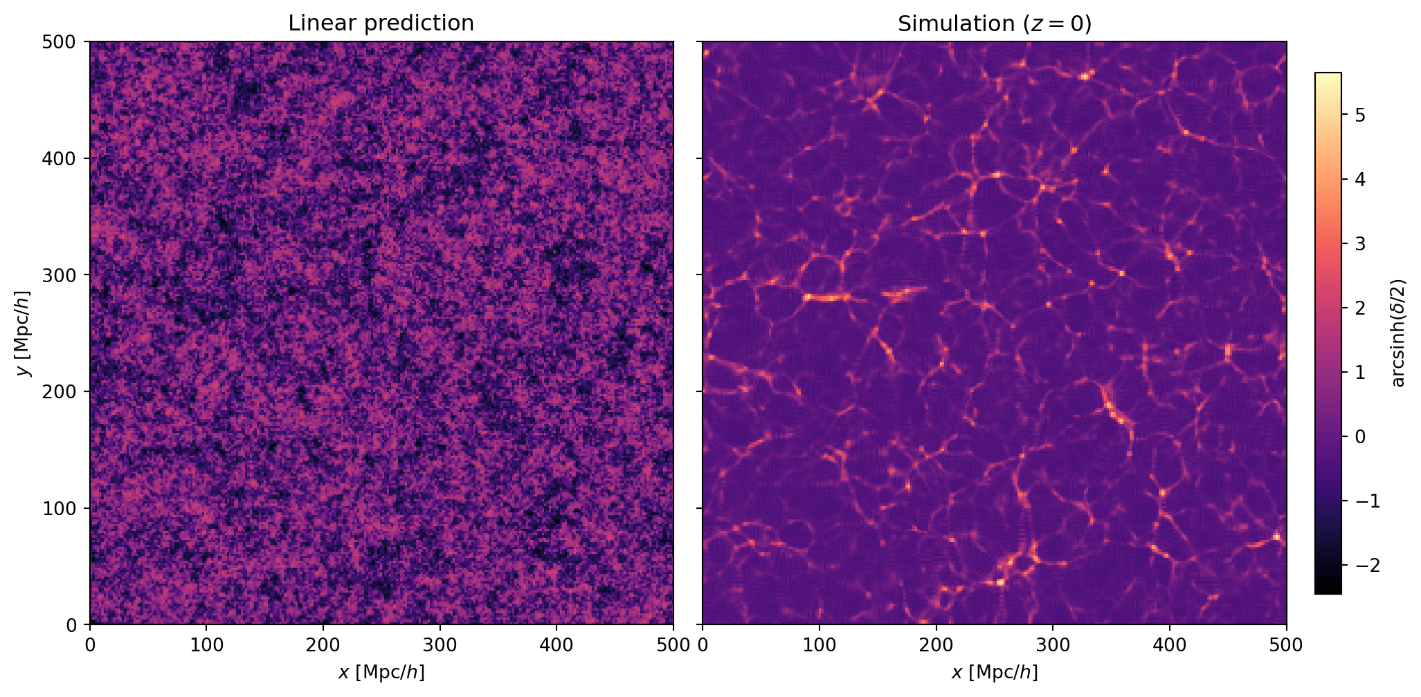
#| label: fig-linear-vs-nonlinear
#| fig-cap: "Comparison of the linear density field (left) and the nonlinear
#| simulation (right) at $z = 0$. The linear field is a Gaussian random
#| field — smooth, with modest fluctuations around zero. The simulation
#| has collapsed this into the cosmic web: thin filaments, dense nodes,
#| and empty voids that have no counterpart in the linear field."
# Linear prediction: delta_0 is already the z=0 field (D_+(1) = 1 for EdS)
delta_linear = delta0_z0

# Nonlinear: CIC deposit of z=0 particles
delta_sim = deposit_to_delta(snapshots[0]['pos'], Ng, L)

# Take a slice
sl = Ng // 2

fig, axes = plt.subplots(1, 2, figsize=(14, 6),
                         gridspec_kw={'wspace': 0.05})

# Common color scale
vmin = arcsinh_scale(delta_linear[:, :, sl]).min()
vmax = arcsinh_scale(delta_sim[:, :, sl]).max()

for ax, delta, title in zip(
    axes,
    [delta_linear, delta_sim],
    ['Linear prediction', 'Simulation ($z = 0$)']
):
    im = ax.imshow(
        arcsinh_scale(delta[:, :, sl]).T,
        origin='lower',
        extent=[0, L, 0, L],
        cmap='magma',
        vmin=vmin, vmax=vmax
    )
    ax.set_xlabel('$x$ [Mpc/$h$]')
    ax.set_title(title)

axes[0].set_ylabel('$y$ [Mpc/$h$]')
axes[1].set_yticklabels([])

plt.colorbar(im, ax=axes, label=r'$\mathrm{arcsinh}(\delta/2)$',
             shrink=0.85, pad=0.02)
plt.show()
```
The contrast between the two panels is striking. The linear density field
is a Gaussian random field: the fluctuations are modest ($|\delta| \lesssim 1$),
the distribution is symmetric around zero, and there is no distinct
"web-like" structure — just a random fluctuation field.
The simulation tells a very different story. Nonlinear gravitational
evolution has reshaped the density field into the cosmic web:
- **Filaments** — thin, elongated structures where matter has streamed
inward from both sides.
- **Nodes** — dense concentrations at the intersections of filaments,
where halos form.
- **Voids** — large, nearly empty regions that have been evacuated as
matter drains onto the surrounding filaments.
None of these features exist in the linear field. They are entirely the
product of nonlinear gravitational collapse. The linear field and the
simulation share the same Fourier phases — the *locations* of future
structures are encoded in the initial conditions — but the *morphology*
of the cosmic web is a nonlinear phenomenon.
The one-point distribution of $\delta$ makes this even clearer.
```{python}
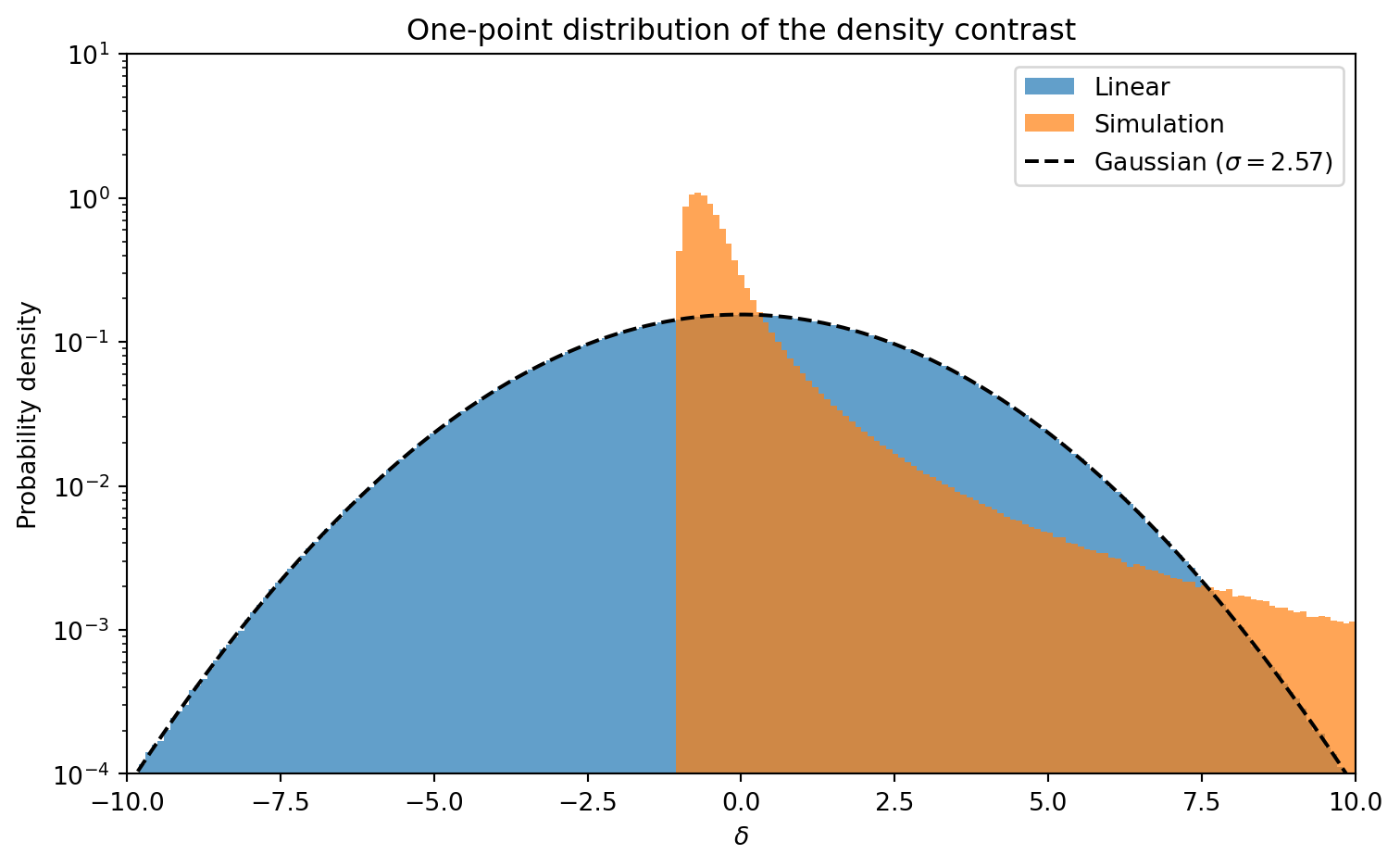
#| label: fig-delta-histogram
#| fig-cap: "Distribution of the overdensity $\\delta$ for the linear field
#| (blue) and the simulation (orange) at $z = 0$. The linear field is
#| an almost perfect Gaussian centered at zero. The nonlinear field has
#| developed a sharp cutoff near $\\delta = -1$ (voids cannot go below
#| $\\rho = 0$) and a heavy positive tail from collapsed structures."
fig, ax = plt.subplots(figsize=(8, 5))

bins = np.linspace(-10, 10, 200)
ax.hist(delta_linear.ravel(), bins=bins, density=True, alpha=0.7,
        label='Linear', histtype='stepfilled')
ax.hist(delta_sim.ravel(), bins=bins, density=True, alpha=0.7,
        label='Simulation', histtype='stepfilled')

# Overplot Gaussian with same variance as linear field
sigma_lin = np.std(delta_linear)
x = np.linspace(-10, 10, 500)
ax.plot(x, np.exp(-x**2 / (2 * sigma_lin**2)) / (sigma_lin * np.sqrt(2 * np.pi)),
        'k--', lw=1.5, label=f'Gaussian ($\\sigma = {sigma_lin:.2f}$)')

ax.set_xlabel(r'$\delta$')
ax.set_ylabel('Probability density')
ax.set_xlim(-10, 10)
ax.set_yscale('log')
ax.set_ylim(1e-4, 10)
ax.legend()
ax.set_title('One-point distribution of the density contrast')
plt.tight_layout()
plt.show()
```
The linear field follows the Gaussian prediction almost exactly. The
nonlinear distribution is strikingly different: it is bounded below by
$\delta = -1$ (density cannot go negative), and the positive tail extends
to $\delta \gg 1$ from collapsed halos. This non-Gaussianity is generated
entirely by gravity — the initial conditions were Gaussian by construction.
::: {.callout-note}
## $\delta < -1$ in the Linear Field
The linear density field shows values below $\delta = -1$, which would
correspond to negative physical density — clearly unphysical. This happens
because the linear field is an *extrapolation*: we took the initial
perturbations at $z = 49$ and scaled them to $z = 0$ using the linear
growth factor $D_+(a) = a$, without accounting for the fact that nonlinear
effects prevent real voids from reaching $\delta = -1$. The linear
prediction is only valid where $|\delta| \ll 1$; by $z = 0$ the rms
fluctuations are of order unity and linear theory has broken down.
:::
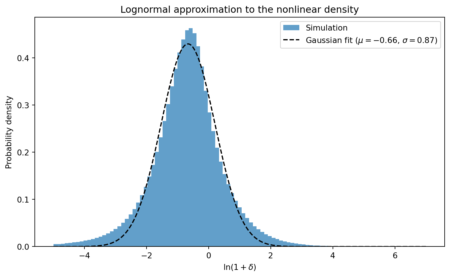
A useful empirical observation: the nonlinear density field is approximately
**lognormal** — that is, $\ln(1 + \delta)$ is roughly Gaussian distributed.
```{python}
#| label: fig-lognormal
#| fig-cap: "Distribution of $\\ln(1 + \\delta)$ for the nonlinear density
#| field at $z = 0$. The approximately Gaussian shape confirms that the
#| nonlinear density is close to lognormally distributed. The dashed line
#| shows a Gaussian fit."
# log(1 + delta) for cells with positive density
rho_flat = (1 + delta_sim).ravel()
mask = rho_flat > 0
log_rho = np.log(rho_flat[mask])

fig, ax = plt.subplots(figsize=(8, 5))

bins = np.linspace(-5, 7, 100)
ax.hist(log_rho, bins=bins, density=True, alpha=0.7,
        label='Simulation', histtype='stepfilled')

# Fit Gaussian to the histogram (curve_fit to the peak, not just mean/std)
from scipy.optimize import curve_fit
hist_vals, bin_edges_fit = np.histogram(log_rho, bins=bins, density=True)
bin_centers_fit = 0.5 * (bin_edges_fit[:-1] + bin_edges_fit[1:])
gauss = lambda x, a, mu, sigma: a * np.exp(-(x - mu)**2 / (2 * sigma**2))
popt, _ = curve_fit(gauss, bin_centers_fit, hist_vals, p0=[0.4, -0.5, 1.0])
x = np.linspace(-5, 7, 500)
ax.plot(x, gauss(x, *popt), 'k--', lw=1.5,
        label=f'Gaussian fit ($\\mu = {popt[1]:.2f}$, $\\sigma = {popt[2]:.2f}$)')

ax.set_xlabel(r'$\ln(1 + \delta)$')
ax.set_ylabel('Probability density')
ax.legend()
ax.set_title('Lognormal approximation to the nonlinear density')
plt.tight_layout()
plt.show()
```
## Power Spectrum Measurement
The power spectrum $P(k)$ quantifies the amplitude of density fluctuations
as a function of scale. We defined `measure_pk` above using the DFT
conventions from Lecture 20: $\hat{\delta}_\text{cont}(\mathbf{k}) = h^3
\hat{\delta}_\text{DFT}(\mathbf{k})$, so
$$
P(k) = \frac{1}{V} |\hat{\delta}_\text{cont}(\mathbf{k})|^2
= \frac{h^6}{V} |\hat{\delta}_\text{DFT}(\mathbf{k})|^2
$$
averaged over spherical shells in $k$.
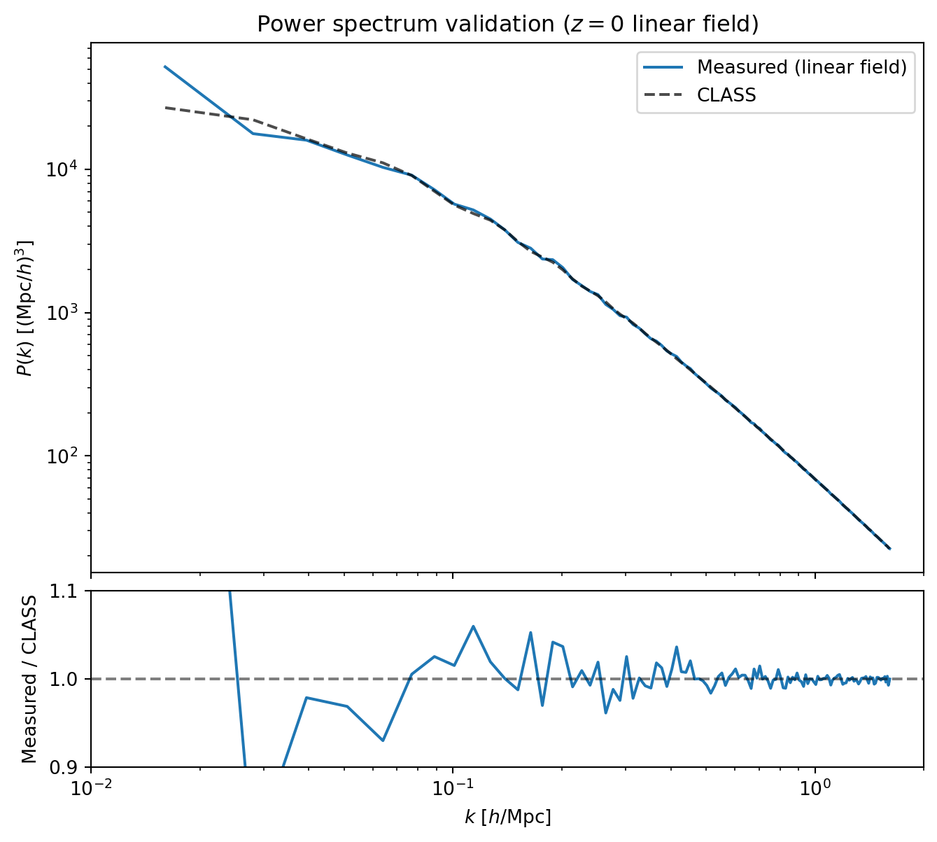
### Validating the Initial Conditions
As a first check, we measure $P(k)$ from the linear density field used to
generate the ICs and compare it to the input CLASS power spectrum. By
construction, the field was built by coloring white noise with
$\sqrt{P(k)}$ from CLASS, so the *expectation value* of the measured $P(k)$
equals CLASS. But any single realization fluctuates around this expectation
— especially at low $k$ where there are few modes per bin. This comparison
validates both that `measure_pk` works correctly and gives a first look
at sample variance.
```{python}
#| label: fig-pk-ic-validation
#| fig-cap: "Validation of the initial conditions and power spectrum
#| measurement. The measured $P(k)$ from the $z = 0$ linear density
#| field (blue) agrees with the input CLASS power spectrum (black dashed).
#| The lower panel shows the ratio, confirming percent-level agreement
#| across the resolved range."
# Measure P(k) from the z=0 linear density field (D_+(1) = 1 for EdS)
k_meas, pk_ic, counts_ic = measure_pk(delta0_z0, kgrid)

# CLASS at z=0
pk_class_ic = pk_of_k(np.array(k_meas))

fig, (ax1, ax2) = plt.subplots(2, 1, figsize=(8, 7),
                                gridspec_kw={'height_ratios': [3, 1], 'hspace': 0.05})

ax1.loglog(k_meas, pk_ic, 'C0-', lw=1.5, label='Measured (linear field)')
ax1.loglog(k_meas, pk_class_ic, 'k--', lw=1.5, alpha=0.7, label='CLASS')
ax1.set_ylabel(r'$P(k)$ [(Mpc/$h$)$^3$]')
ax1.set_xlim(0.01, 2)
ax1.legend()
ax1.set_xticklabels([])
ax1.set_title('Power spectrum validation ($z = 0$ linear field)')

ratio_ic = np.array(pk_ic) / pk_class_ic
ax2.semilogx(k_meas, ratio_ic, 'C0-', lw=1.5)
ax2.axhline(1.0, color='k', ls='--', alpha=0.5)
ax2.set_xlabel(r'$k$ [$h$/Mpc]')
ax2.set_ylabel('Measured / CLASS')
ax2.set_xlim(0.01, 2)
ax2.set_ylim(0.9, 1.1)

plt.show()
```
### Nonlinear Power Spectrum at $z = 0$
Now we compare the simulation's power spectrum at $z = 0$ to the linear
field from the ICs.
```{python}
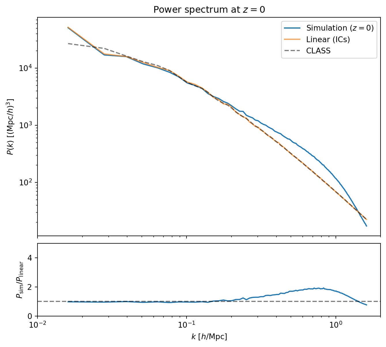
#| label: fig-pk-z0
#| fig-cap: "Power spectrum at $z = 0$: simulation (blue) versus the
#| linear IC field (orange) and CLASS (black dashed). The simulation
#| tracks the linear prediction on large scales, shows nonlinear
#| enhancement at intermediate scales, and falls below at high $k$ due
#| to the PM force resolution limit."
# Measure P(k) from z=0 simulation
k_meas, pk_z0, counts_z0 = measure_pk(delta_sim, kgrid)

# CLASS P(k) at z=0
pk_class_z0 = pk_of_k(np.array(k_meas))

fig, (ax1, ax2) = plt.subplots(2, 1, figsize=(8, 7),
                                gridspec_kw={'height_ratios': [3, 1], 'hspace': 0.05})

ax1.loglog(k_meas, pk_z0, 'C0-', lw=1.5, label='Simulation ($z = 0$)')
ax1.loglog(k_meas, pk_ic, 'C1-', lw=1.5, alpha=0.7, label='Linear (ICs)')
ax1.loglog(k_meas, pk_class_z0, 'k--', lw=1.5, alpha=0.5, label='CLASS')
ax1.set_ylabel(r'$P(k)$ [(Mpc/$h$)$^3$]')
ax1.set_xlim(0.01, 2)
ax1.legend()
ax1.set_xticklabels([])
ax1.set_title('Power spectrum at $z = 0$')

ratio_z0 = np.array(pk_z0) / np.array(pk_ic)
ax2.semilogx(k_meas, ratio_z0, 'C0-', lw=1.5)
ax2.axhline(1.0, color='k', ls='--', alpha=0.5)
ax2.set_xlabel(r'$k$ [$h$/Mpc]')
ax2.set_ylabel(r'$P_\mathrm{sim} / P_\mathrm{linear}$')
ax2.set_xlim(0.01, 2)
ax2.set_ylim(0, 5)

plt.show()
```
The ratio plot reveals three regimes:
- **Large scales** ($k \lesssim 0.1\,h$/Mpc): the simulation tracks linear
theory — perturbations on these scales are still in the linear regime
at $z = 0$.
- **Intermediate scales** ($0.1 \lesssim k \lesssim 0.5\,h$/Mpc): the
ratio exceeds unity — nonlinear mode coupling transfers power from large
scales to small scales, boosting $P(k)$ above the linear prediction.
- **Small scales** ($k \gtrsim 0.5\,h$/Mpc): the ratio turns over and
eventually drops below unity. This is not physical — it is the PM
resolution limit. The CIC mass assignment and finite grid smooth the
force on scales smaller than a few grid cells, suppressing small-scale
power.
::: {.callout-note}
## PM Resolution
The PM method resolves forces down to scales of order the grid spacing
$h = L / N_g$. In Fourier space, the CIC window function and the discrete
Laplacian both suppress power near the Nyquist frequency
$k_\text{Ny} = \pi N_g / L$. Production codes use TreePM or P$^3$M methods
to supplement the grid-based force with direct particle-particle
interactions on small scales, eliminating this artificial suppression.
:::
## Growth Factor Evolution
In linear theory, all Fourier modes grow at the same rate: $P(k, a) =
D_+(a)^2 \, P(k, a_\text{init}) / D_+(a_\text{init})^2$. For EdS,
$D_+(a) = a$, so the ratio $P(k, a) / P(k, a_\text{init})$ should equal
$(a / a_\text{init})^2$ for modes in the linear regime. Nonlinear modes
grow faster than this prediction.
We measure $P(k)$ at each of our saved snapshots ($z = 9, 4, 1, 0$) and
first show the full power spectra, then track the growth of individual
$k$-bins.
```{python}
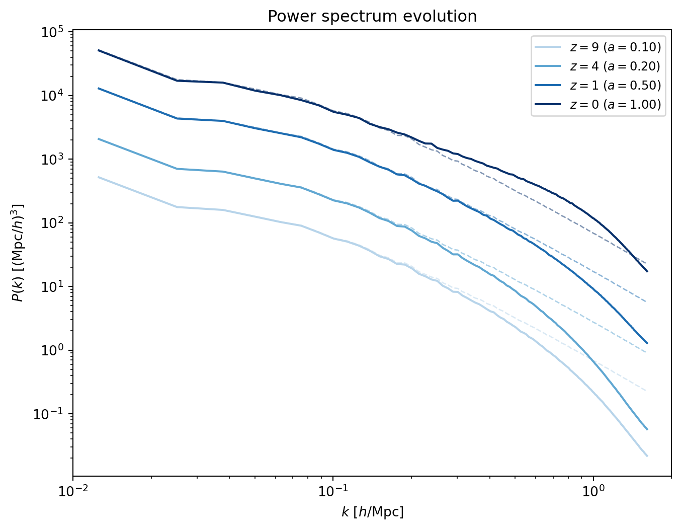
#| label: fig-pk-evolution
#| fig-cap: "Power spectra at four redshifts, from $z = 9$ (lightest) to
#| $z = 0$ (darkest). Solid lines are the simulation; dashed lines show
#| the linear prediction (IC field scaled by $(a/a_i)^2$). At early times
#| the two agree; by $z = 0$ nonlinear growth boosts intermediate scales
#| while PM resolution and the CIC window suppress high $k$."
# Measure P(k) at each snapshot
pk_snapshots = {}
for z_snap in z_snapshots:
    delta_snap = deposit_to_delta(snapshots[z_snap]['pos'], Ng, L)
    _, pk_snap, _ = measure_pk(delta_snap, kgrid)
    pk_snapshots[z_snap] = pk_snap

# P(k) at the initial conditions (reference)
_, pk_init, _ = measure_pk(deposit_to_delta(pos_ic, Ng, L), kgrid)

k_centers = np.array(kgrid['k_centers'])

fig, ax = plt.subplots(figsize=(8, 6))

# Snapshots with increasing darkness, plus scaled IC prediction
colors = plt.cm.Blues(np.linspace(0.3, 1.0, len(z_snapshots)))
for i, z_snap in enumerate(z_snapshots):
    a_snap = snapshots[z_snap]['a']
    # Scaled IC: P(k, a) = P_IC(k) * D+(a)^2 = P_IC(k) * a^2  (EdS, IC is at z=0)
    pk_scaled_ic = np.array(pk_ic) * a_snap**2
    ax.loglog(k_centers, pk_scaled_ic, color=colors[i], lw=1, ls='--', alpha=0.5)
    ax.loglog(k_centers, pk_snapshots[z_snap], color=colors[i], lw=1.5,
              label=f'$z = {z_snap}$ ($a = {a_snap:.2f}$)')

ax.set_xlabel(r'$k$ [$h$/Mpc]')
ax.set_ylabel(r'$P(k)$ [(Mpc/$h$)$^3$]')
ax.set_xlim(0.01, 2)
ax.legend(fontsize=9)
ax.set_title('Power spectrum evolution')
plt.show()
```
Now we track the growth of specific $k$-bins as a function of scale factor,
normalized by their initial values.
```{python}
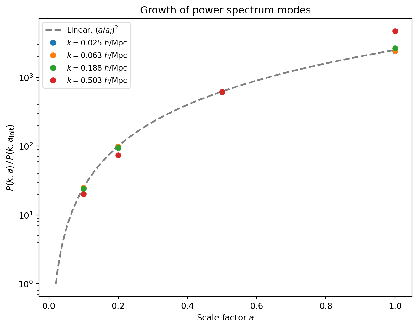
#| label: fig-growth-factor
#| fig-cap: "Growth of the power spectrum with scale factor for several
#| $k$-bins. The dashed line shows the EdS linear prediction
#| $(a / a_i)^2$. Large-scale modes (low $k$) track linear theory
#| closely, while small-scale modes grow faster due to nonlinear
#| mode coupling."
k_fund = 2 * np.pi / L
k_targets = [2 * k_fund, 5 * k_fund, 15 * k_fund, 40 * k_fund]

fig, ax = plt.subplots(figsize=(8, 6))

# EdS prediction: (a / a_init)^2
a_theory = np.linspace(a_init, 1.0, 200)
ax.plot(a_theory, (a_theory / a_init)**2, 'k--', lw=2, alpha=0.5,
        label=r'Linear: $(a/a_i)^2$')

for ik_target, k_target in enumerate(k_targets):
    idx_k = np.argmin(np.abs(k_centers - k_target))
    k_actual = k_centers[idx_k]
    pk_ref = float(pk_init[idx_k])

    a_vals = []
    growth_vals = []
    for z_snap in z_snapshots:
        a_snap = snapshots[z_snap]['a']
        a_vals.append(a_snap)
        growth_vals.append(float(pk_snapshots[z_snap][idx_k]) / pk_ref)

    ax.plot(a_vals, growth_vals, 'o', color=f'C{ik_target}',
            label=f'$k = {k_actual:.3f}$ $h$/Mpc', ms=6)

ax.set_xlabel('Scale factor $a$')
ax.set_ylabel(r'$P(k, a) \,/\, P(k, a_\mathrm{init})$')
ax.set_title('Growth of power spectrum modes')
ax.set_yscale('log')
ax.legend(fontsize=9)
plt.show()
```
The large-scale modes ($k \lesssim 0.05\,h$/Mpc) follow the linear
prediction $(a/a_i)^2$ almost exactly — these modes are still in the
linear regime even at $z = 0$. At higher $k$, the growth exceeds the
linear prediction: nonlinear mode coupling (the transfer of power from
large to small scales) accelerates the growth of small-scale power. This
is the same nonlinear enhancement we saw in the $P(k)$ ratio plot, but
now tracked as a function of time.
## Redshift-Space Density Field
In observations, we do not measure the true (real-space) positions of
galaxies. Instead, we infer distances from redshifts, which include a
contribution from peculiar velocities. This maps the real-space position
$\mathbf{x}$ to a **redshift-space position** $\mathbf{s}$:
$$
\mathbf{s} = \mathbf{x} + \frac{v_{\text{pec},\parallel}}{aH} \hat{\mathbf{n}}
$$
where $\hat{\mathbf{n}}$ is the line-of-sight (LOS) direction and
$v_{\text{pec},\parallel}$ is the peculiar velocity component along it.
In the **plane-parallel approximation** (valid when the survey is far enough
away that all lines of sight are nearly parallel), we pick a fixed LOS
direction — here the $z$-axis. In our code units at $a = 1$ (EdS,
$H_0 = 1$, $m = 1$): the momentum $\mathbf{p} = a^2 \dot{\mathbf{x}}$
equals $a \, \mathbf{v}_\text{pec}$, so at $a = 1$, $\mathbf{p} =
\mathbf{v}_\text{pec}$ and $aH = 1$, giving simply
$$
s_z = x_z + p_z, \qquad s_x = x_x, \qquad s_y = x_y
$$
```{python}
# Compute redshift-space positions at z=0
pos_z0 = snapshots[0]['pos']
mom_z0 = snapshots[0]['mom']

# RSD displacement along z-axis: s_z = x_z + p_z (at a=1, H_0=1, m=1)
pos_rsd = pos_z0.at[:, 2].add(mom_z0[:, 2])
pos_rsd = pos_rsd % L  # periodic wrapping

# Deposit both real-space and redshift-space onto the grid
delta_real = deposit_to_delta(pos_z0, Ng, L)
delta_rsd = deposit_to_delta(pos_rsd, Ng, L)
```
### Slices Parallel to the LOS
Since the RSD displacement is along the $z$-axis, we need a slice that
includes $z$ to see the effect. We show an $x$–$z$ slice at fixed $y$,
comparing real space and redshift space side by side, followed by a
zoomed-in view of a dense region.
```{python}
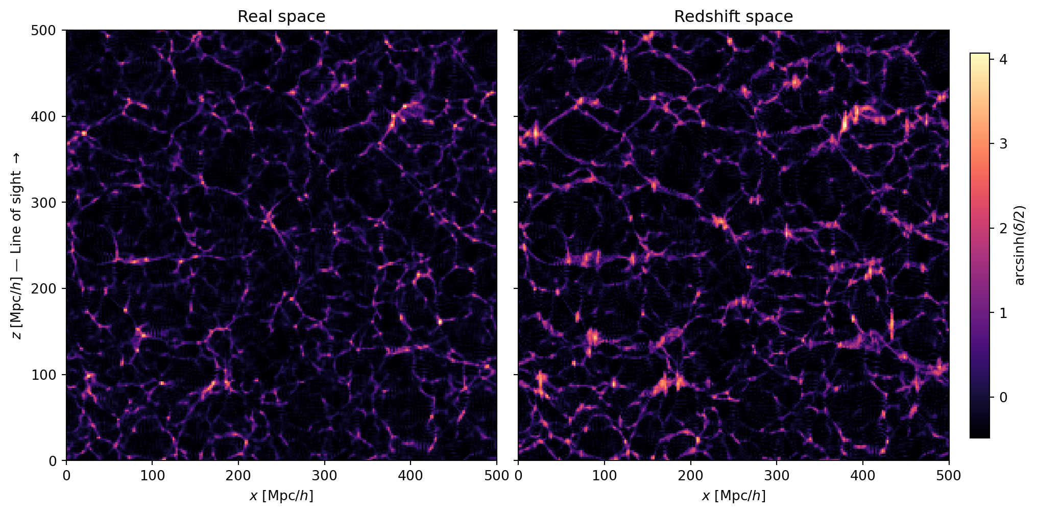
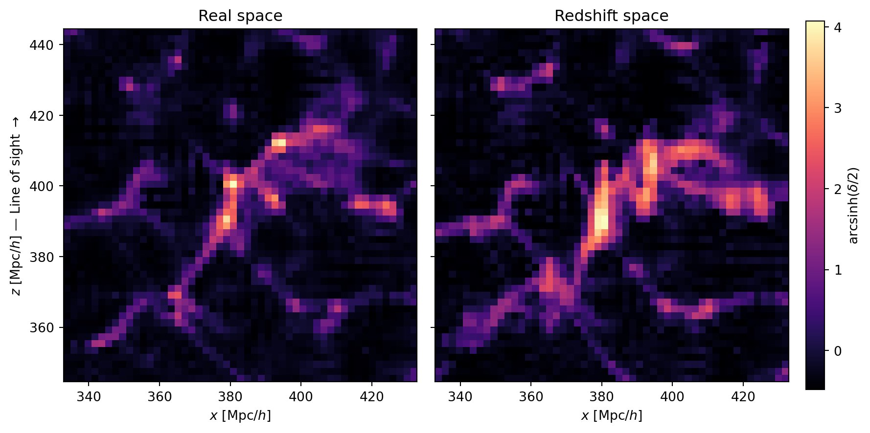
#| label: fig-rsd-slices
#| fig-cap: "Real-space (left) and redshift-space (right) density in an
#| $x$–$z$ slice. The vertical axis is the line of sight. Coherent
#| infall squashes large-scale structures along $z$ (Kaiser effect),
#| while virialized motions in clusters elongate them (Fingers of God)."
sl = Ng // 2

fig, axes = plt.subplots(1, 2, figsize=(14, 6),
                         gridspec_kw={'wspace': 0.05})

for ax, delta, title in zip(
    axes,
    [delta_real, delta_rsd],
    ['Real space', 'Redshift space']
):
    im = ax.imshow(
        arcsinh_scale(delta[:, sl, :]).T,
        origin='lower',
        extent=[0, L, 0, L],
        cmap='magma',
    )
    ax.set_xlabel('$x$ [Mpc/$h$]')
    ax.set_title(title)

axes[0].set_ylabel(r'$z$ [Mpc/$h$] — Line of sight $\rightarrow$')
axes[1].set_yticklabels([])

plt.colorbar(im, ax=axes, label=r'$\mathrm{arcsinh}(\delta/2)$',
             shrink=0.85, pad=0.02)
plt.show()
```
Now we zoom in on a dense region to see the Fingers of God more clearly.
```{python}
#| label: fig-rsd-zoom
#| fig-cap: "Zoomed view of a $100 \\times 100$ (Mpc/$h$)$^2$ region in
#| real space (left) and redshift space (right). Dense clusters that
#| appear compact in real space are stretched along the line of sight
#| (vertical) in redshift space — the classic Fingers of God."
# Find a dense region to zoom into: look for the peak in this slice
slice_data = np.array(delta_real[:, sl, :])
# Smooth to find a broad peak, not a single cell
from scipy.ndimage import uniform_filter
smoothed = uniform_filter(slice_data, size=10)
peak_idx = np.unravel_index(smoothed.argmax(), smoothed.shape)
h_cell = L / Ng

# Center the zoom on the peak, 100 Mpc/h box
zoom_size = 100.0  # Mpc/h
x_center = peak_idx[0] * h_cell
z_center = peak_idx[1] * h_cell
x_lo = max(0, x_center - zoom_size / 2)
x_hi = min(L, x_center + zoom_size / 2)
z_lo = max(0, z_center - zoom_size / 2)
z_hi = min(L, z_center + zoom_size / 2)

# Grid indices for the zoom
ix_lo = int(x_lo / h_cell)
ix_hi = int(x_hi / h_cell)
iz_lo = int(z_lo / h_cell)
iz_hi = int(z_hi / h_cell)

fig, axes = plt.subplots(1, 2, figsize=(12, 6),
                         gridspec_kw={'wspace': 0.05})

for ax, delta, title in zip(
    axes,
    [delta_real, delta_rsd],
    ['Real space', 'Redshift space']
):
    im = ax.imshow(
        arcsinh_scale(delta[ix_lo:ix_hi, sl, iz_lo:iz_hi]).T,
        origin='lower',
        extent=[x_lo, x_hi, z_lo, z_hi],
        cmap='magma',
    )
    ax.set_xlabel('$x$ [Mpc/$h$]')
    ax.set_title(title)
    ax.set_aspect('equal')

axes[0].set_ylabel(r'$z$ [Mpc/$h$] — Line of sight $\rightarrow$')
axes[1].set_yticklabels([])

plt.colorbar(im, ax=axes, label=r'$\mathrm{arcsinh}(\delta/2)$',
             shrink=0.85, pad=0.02)
plt.show()
```
Two effects are at work in these slices:
- **Kaiser squashing**: large-scale overdensities appear compressed along
the $z$-axis in redshift space. This is because matter is falling
coherently toward the overdensity — the infalling material on the near
side has a peculiar velocity *toward* us (reducing its redshift), while
material on the far side moves *away* (increasing its redshift). Both
shifts push the material closer together in redshift space.
- **Fingers of God**: dense clusters appear elongated along $z$. Inside a
virialized halo, galaxies have large random velocities that scatter their
redshifts, smearing the cluster along the line of sight.
The Kaiser effect is subtle in individual slices — it is a large-scale
coherent compression that is difficult to see by eye. In the next section,
we will measure the power spectrum *multipoles*, which quantify the
anisotropy statistically and make the Kaiser signal unambiguous.
::: {.callout-note}
## Plane-Parallel Approximation
We assumed a single, fixed line of sight for the entire box. This is the
plane-parallel (or distant-observer) approximation, valid when the box
subtends a small angle on the sky. For a real survey covering a large
fraction of the sky, the LOS varies across the volume and one must account
for the changing projection direction — the so-called "wide-angle" effects.
:::
### 2D Correlation Function
A more quantitative view of the anisotropy comes from the two-point
correlation function $\xi(r_\perp, r_\parallel)$, where $r_\parallel$ is
the separation along the LOS and $r_\perp$ is perpendicular to it. We
compute this by FFT: $\xi(\mathbf{r}) = \text{IFFT}(|\hat{\delta}(\mathbf{k})|^2) / N_g^3$.
In real space, $\xi$ depends only on $|\mathbf{r}|$ — the contours are
circular. In redshift space, the Kaiser effect squashes the contours along
$r_\parallel$ on large scales (coherent infall makes structures appear
closer together along the LOS), while the Fingers of God elongate them
on small scales.
```{python}
#| label: fig-2d-corr
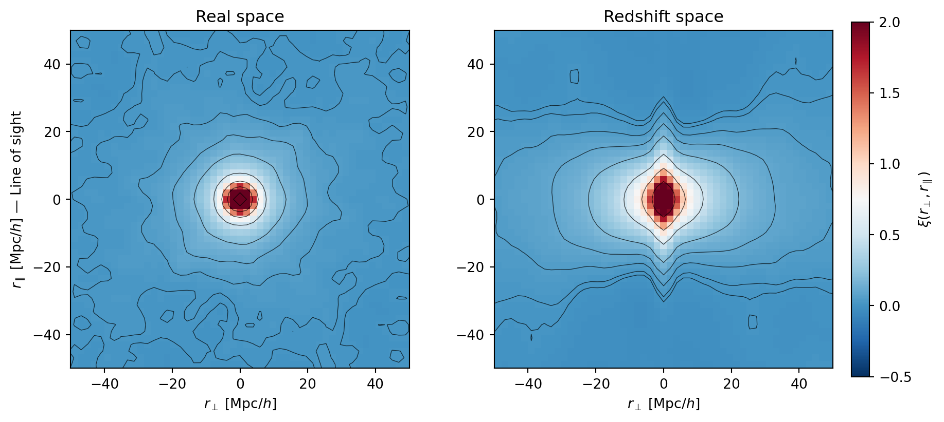
#| fig-cap: "Two-point correlation function $\\xi(r_\\perp, r_\\parallel)$
#| in real space (left) and redshift space (right). In real space the
#| contours are nearly circular (isotropic). In redshift space, the
#| Kaiser effect squashes the contours along $r_\\parallel$ at large
#| separations, while the Fingers of God elongate them at small
#| separations."
def compute_xi_2d(delta, Ng):
    """Compute 2D correlation function xi(r_perp, r_parallel) via FFT."""
    delta_hat = np.fft.fftn(np.array(delta))
    power = np.abs(delta_hat)**2
    xi_3d = np.fft.ifftn(power).real / Ng**3

    # Extract the r_y = 0 slice: xi(r_x, 0, r_z) = xi(r_perp, r_parallel)
    # Use fftshift to center r=0
    xi_slice = np.fft.fftshift(xi_3d[:, 0, :])
    return xi_slice

xi_real = compute_xi_2d(delta_real, Ng)
xi_rsd = compute_xi_2d(delta_rsd, Ng)

# Coordinate arrays for the shifted grid
h_cell = L / Ng
r_vals = np.fft.fftshift(np.fft.fftfreq(Ng, d=1.0/L))

fig, axes = plt.subplots(1, 2, figsize=(12, 5.5),
                         gridspec_kw={'wspace': 0.25})

rmax = 50  # Mpc/h — zoom in to see the structure
levels = np.array([0.01, 0.02, 0.05, 0.1, 0.2, 0.5, 1.0, 2.0, 5.0])

for ax, xi, title in zip(axes, [xi_real, xi_rsd],
                          ['Real space', 'Redshift space']):
    im = ax.pcolormesh(r_vals, r_vals, xi.T, cmap='RdBu_r',
                       vmin=-0.5, vmax=2.0, shading='auto')
    ax.contour(r_vals, r_vals, xi.T, levels=levels,
               colors='k', linewidths=0.5, alpha=0.7)
    ax.set_xlim(-rmax, rmax)
    ax.set_ylim(-rmax, rmax)
    ax.set_xlabel(r'$r_\perp$ [Mpc/$h$]')
    ax.set_title(title)
    ax.set_aspect('equal')

axes[0].set_ylabel(r'$r_\parallel$ [Mpc/$h$] — Line of sight')
plt.colorbar(im, ax=axes, label=r'$\xi(r_\perp, r_\parallel)$',
             shrink=0.85, pad=0.02)
plt.show()
```
The contour plot makes the RSD anisotropy unmistakable. In real space, the
contours of constant $\xi$ are roughly circular — the clustering is
isotropic. In redshift space, two distortions are visible:
- At **large separations**, the contours are squashed along $r_\parallel$
(they are wider in $r_\perp$ than in $r_\parallel$). This is the Kaiser
effect: coherent infall compresses structures along the LOS.
- At **small separations**, the contours are elongated along $r_\parallel$.
This is the Fingers of God: random velocities inside halos smear out
the clustering along the LOS.
## RSD Power Spectrum Multipoles
### Theory: Kaiser Formula
In linear theory, the redshift-space power spectrum depends on the angle
$\mu = \hat{\mathbf{k}} \cdot \hat{\mathbf{n}}$ between the wavevector and
the line of sight:
$$
P^s(k, \mu) = (1 + \beta \mu^2)^2 \, P(k)
$$
where $\beta = f/b$, $f = d\ln D_+ / d\ln a$ is the growth rate, $b$ is
the linear bias, and $P(k)$ is the real-space power spectrum. For EdS dark
matter: $f = 1$ and $b = 1$, so $\beta = 1$.
Expanding in Legendre polynomials $\mathcal{L}_\ell(\mu)$, the multipoles
are
$$
P_\ell(k) = \frac{2\ell + 1}{2} \int_{-1}^{1} P^s(k, \mu) \, \mathcal{L}_\ell(\mu) \, d\mu
$$
For the Kaiser formula with $\beta = 1$:
$$
P_0(k) = \left(1 + \frac{2}{3}\beta + \frac{1}{5}\beta^2\right) P(k) = \frac{28}{15} P(k)
$$
$$
P_2(k) = \left(\frac{4}{3}\beta + \frac{4}{7}\beta^2\right) P(k) = \frac{40}{21} P(k)
$$
### Measuring Multipoles
We measure $P(k, \mu)$ on a 2D grid, then integrate over $\mu$ with
Legendre weights. The `kgrid` already stores the bin indices for both
$k$ and $|\mu|$.
```{python}
#| code-fold: true
#| code-summary: "Power spectrum multipole measurement"
@partial(jax.jit, static_argnums=(3, 4))
def _bin_power_2d(power_flat, ik, imu, n_k, n_mu):
    """Scatter-add power into 2D (k, |mu|) bins."""
    # Clamp ik to valid range for 2D index computation;
    # out-of-range entries are dropped by mode='drop'
    valid = (ik >= 0) & (ik < n_k)
    idx_2d = jnp.where(valid, ik * n_mu + imu, -1)
    n_total = n_k * n_mu
    pk_sum = jnp.zeros(n_total).at[idx_2d].add(power_flat, mode='drop')
    counts = jnp.zeros(n_total).at[idx_2d].add(jnp.ones_like(power_flat), mode='drop')
    pk_2d = jnp.where(counts > 0, pk_sum / counts, 0.0)
    return pk_2d.reshape(n_k, n_mu), counts.reshape(n_k, n_mu)

def measure_pk_multipoles(delta, kgrid, ells=(0, 2)):
    """
    Measure power spectrum multipoles P_ell(k).

    Parameters
    ----------
    delta : array (Ng, Ng, Ng)
        Overdensity field (real or redshift space).
    kgrid : dict
        Output of make_k_grid.
    ells : tuple of int
        Multipole orders to compute.

    Returns
    -------
    k_centers : array
    multipoles : dict mapping ell -> P_ell(k) array
    """
    delta_hat = jnp.fft.fftn(jnp.asarray(delta))
    power_flat = jnp.abs(delta_hat).ravel()**2 * kgrid['norm']

    n_k = kgrid['n_k_bins']
    n_mu = kgrid['n_mu_bins']

    pk_2d, counts_2d = _bin_power_2d(
        power_flat, kgrid['ik'], kgrid['imu'], n_k, n_mu
    )

    pk_2d = np.array(pk_2d)
    counts_2d = np.array(counts_2d)
    mu_centers = np.array(kgrid['mu_centers'])
    dmu = mu_centers[1] - mu_centers[0]

    multipoles = {}
    for ell in ells:
        if ell == 0:
            L_ell = np.ones_like(mu_centers)
        elif ell == 2:
            L_ell = 0.5 * (3 * mu_centers**2 - 1)
        else:
            raise ValueError(f"ell={ell} not implemented")

        # P_ell = (2ell+1) * int_0^1 P(k,|mu|) L_ell(mu) dmu
        # (the (2ell+1)/2 from the full [-1,1] integral becomes (2ell+1)
        #  after folding the symmetric integrand onto [0,1])
        integrand = pk_2d * L_ell[np.newaxis, :] * (2 * ell + 1)
        multipoles[ell] = np.sum(integrand * dmu, axis=1)

    return kgrid['k_eff'], multipoles
```
### Single Realization
We measure the monopole $P_0(k)$ and quadrupole $P_2(k)$ from the
redshift-space density field of our single $z = 0$ realization, along with
the real-space $P(k)$ for comparison with the Kaiser prediction.
```{python}
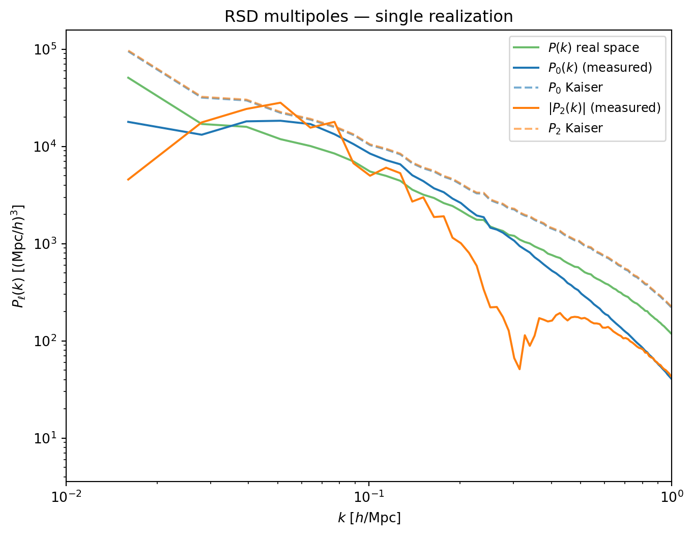
#| label: fig-rsd-multipoles-single
#| fig-cap: "RSD multipoles from a single realization: monopole $P_0(k)$,
#| quadrupole $|P_2(k)|$, and real-space $P(k)$, compared to the Kaiser
#| prediction (dashed). The quadrupole is noisy — a consequence of sample
#| variance from a finite number of modes per $k$-bin."
# Measure multipoles from redshift-space field
k_meas, pells_rsd = measure_pk_multipoles(delta_rsd, kgrid, ells=(0, 2))

# Real-space P(k) for Kaiser prediction
k_meas_real, pk_real, _ = measure_pk(delta_real, kgrid)

# Kaiser prediction (beta = 1 for EdS dark matter)
beta = 1.0
kaiser_0 = (1 + 2*beta/3 + beta**2/5)      # 28/15
kaiser_2 = (4*beta/3 + 4*beta**2/7)         # 40/21
pk_kaiser_0 = kaiser_0 * np.array(pk_real)
pk_kaiser_2 = kaiser_2 * np.array(pk_real)

k_np = np.array(k_meas)
p0 = np.array(pells_rsd[0])
p2 = np.array(pells_rsd[2])

fig, ax = plt.subplots(figsize=(8, 6))

ax.loglog(k_np, np.array(pk_real), 'C2-', lw=1.5, alpha=0.7, label=r'$P(k)$ real space')
ax.loglog(k_np, p0, 'C0-', lw=1.5, label=r'$P_0(k)$ (measured)')
ax.loglog(k_np, pk_kaiser_0, 'C0--', lw=1.5, alpha=0.6, label=r'$P_0$ Kaiser')
ax.loglog(k_np, np.abs(p2), 'C1-', lw=1.5, label=r'$|P_2(k)|$ (measured)')
ax.loglog(k_np, pk_kaiser_2, 'C1--', lw=1.5, alpha=0.6, label=r'$P_2$ Kaiser')
ax.set_xlabel(r'$k$ [$h$/Mpc]')
ax.set_ylabel(r'$P_\ell(k)$ [(Mpc/$h$)$^3$]')
ax.set_xlim(0.01, 1)
ax.legend(fontsize=9)
ax.set_title('RSD multipoles — single realization')

plt.show()
```
The monopole is reasonably well described by the Kaiser formula on large
scales ($k \lesssim 0.2\,h$/Mpc), but the quadrupole is much noisier. This
is not surprising: the quadrupole is a higher-order statistic that requires
more modes to average down the variance. At low $k$, there are very few
modes per spherical shell, and the $\mu$-dependence is poorly sampled.
Notice that $P_2$ actually *exceeds* $P_0$ — the Kaiser coefficients are
$28/15 \approx 1.87$ for the monopole and $40/21 \approx 1.90$ for the
quadrupole when $\beta = 1$. This is a peculiarity of EdS dark matter
($f = 1$, $b = 1$). In a realistic galaxy survey, both $f < 1$ (in $\Lambda$CDM, $f \approx
\Omega_m^{0.55} \lesssim 1$) and $b > 1$ for typical tracers, so $\beta =
f/b$ is well below unity and the quadrupole is much smaller than the
monopole — making it harder to measure and more sensitive to systematic
errors.
At small scales, both multipoles deviate from Kaiser. The Fingers of God
suppress power along the LOS, reducing $P_0$ below the Kaiser prediction.
The quadrupole $P_2$ actually goes negative at high $k$ — the anisotropy
reverses sign as the elongation from FoG dominates over the Kaiser
squashing. (We plot $|P_2|$ on the log scale, so this sign change shows up
as the ratio crossing zero in the lower panel.) The Kaiser formula, which
assumes linear velocities, cannot capture this nonlinear effect.
::: {.callout-note}
## Sample Variance
The scatter in the multipoles — especially $P_2$ — is **sample variance**
(also called cosmic variance). A single realization of a finite box
contains a limited number of independent Fourier modes at each $k$. The
measured power in each bin fluctuates around the true expectation value,
and this scatter is worst at low $k$ where there are fewest modes. In the
next section, we will run an ensemble of simulations to beat down this
variance and extract a clean signal.
:::
### Ensemble of Realizations
To reduce sample variance, we run 10 independent simulations with
different random seeds (but the same cosmology and box parameters). For
each realization, we measure the real-space $P(k)$, the redshift-space
multipoles $P_0(k)$ and $P_2(k)$, and the 2D correlation function.
::: {.callout-important}
## Precomputed Ensemble
The ensemble simulations are too expensive to run inside the notebook.
They were precomputed separately using `scripts/run_ensemble.py` and
cached to `~/data/teaching/ASTR6000-SP26/021-pm-analysis/ensemble/`. To regenerate:
```bash
pixi run python scripts/run_ensemble.py --n-real 10
```
This takes ~15 minutes (10 simulations × ~90s each).
:::
```{python}
# Load ensemble results
ensemble_dir = os.path.join(CACHE_DIR, "ensemble")

pk_real_all = []
p0_all = []
p2_all = []

n_real = 0
while os.path.exists(os.path.join(ensemble_dir, f"real_{n_real:03d}.npz")):
    n_real += 1

print(f"Loading {n_real} realizations from {ensemble_dir}")

for i in range(n_real):
    d = np.load(os.path.join(ensemble_dir, f"real_{i:03d}.npz"))
    pk_real_all.append(d['pk_real'])
    p0_all.append(d['p0'])
    p2_all.append(d['p2'])

# Use k_eff from the notebook's kgrid (consistent with our measure_pk)
k_ens = np.array(kgrid['k_eff'])

pk_real_all = np.array(pk_real_all)
p0_all = np.array(p0_all)
p2_all = np.array(p2_all)

print(f"  k bins: {len(k_ens)}, realizations: {n_real}")
```
#### Spaghetti Plots
First, we overlay all realizations to visualize the scatter.
```{python}
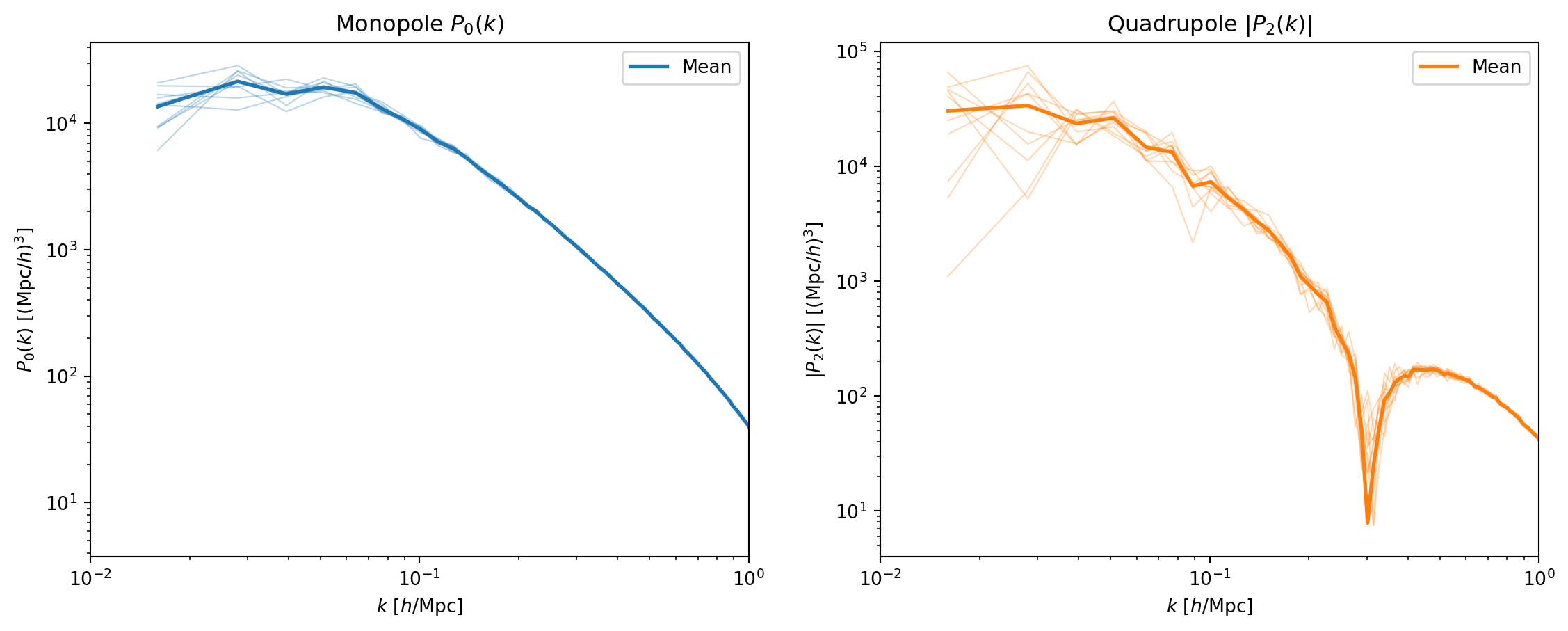
#| label: fig-ensemble-spaghetti
#| fig-cap: "All 10 realizations overplotted for the monopole $P_0(k)$
#| (left) and quadrupole $|P_2(k)|$ (right). The spread between
#| realizations is sample variance — it is largest at low $k$ where
#| there are fewest independent modes."
fig, axes = plt.subplots(1, 2, figsize=(14, 5))

# P0 spaghetti
ax = axes[0]
for i in range(n_real):
    ax.loglog(k_ens, p0_all[i], 'C0-', alpha=0.3, lw=0.8)
ax.loglog(k_ens, np.mean(p0_all, axis=0), 'C0-', lw=2, label='Mean')
ax.set_xlabel(r'$k$ [$h$/Mpc]')
ax.set_ylabel(r'$P_0(k)$ [(Mpc/$h$)$^3$]')
ax.set_xlim(0.01, 1)
ax.set_title(r'Monopole $P_0(k)$')
ax.legend()

# P2 spaghetti
ax = axes[1]
for i in range(n_real):
    ax.loglog(k_ens, np.abs(p2_all[i]), 'C1-', alpha=0.3, lw=0.8)
ax.loglog(k_ens, np.abs(np.mean(p2_all, axis=0)), 'C1-', lw=2, label='Mean')
ax.set_xlabel(r'$k$ [$h$/Mpc]')
ax.set_ylabel(r'$|P_2(k)|$ [(Mpc/$h$)$^3$]')
ax.set_xlim(0.01, 1)
ax.set_title(r'Quadrupole $|P_2(k)|$')
ax.legend()

plt.show()
```
The scatter is dramatically worse for the quadrupole — consistent with
what we saw in the single realization. At $k \lesssim 0.03\,h$/Mpc, the
individual quadrupole measurements jump around wildly, while the monopole
is relatively stable even at the lowest $k$.
#### Mean and Error Bars vs Kaiser
Finally, the ensemble mean with error bars, compared to the Kaiser
prediction. We also show the mean real-space $P(k)$ compared to the
IC linear prediction.
```{python}
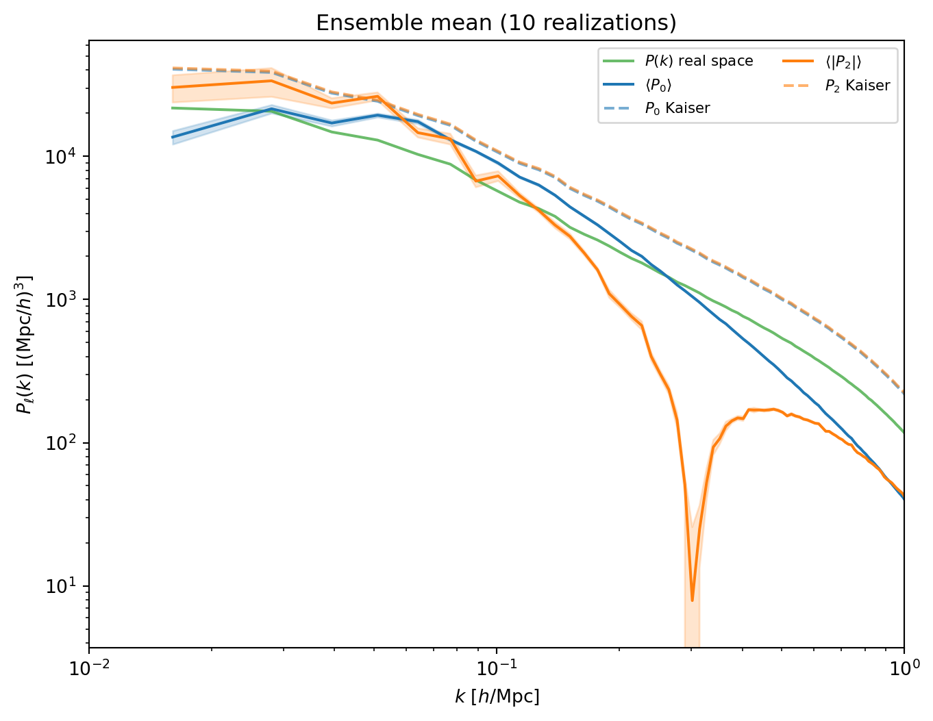
#| label: fig-ensemble-mean
#| fig-cap: "Ensemble mean of $P_0(k)$ and $P_2(k)$ (with standard error
#| shading) compared to the Kaiser prediction (dashed) and the real-space
#| $P(k)$. The Kaiser formula captures the qualitative behavior; deviations
#| at small scales are from Fingers of God and PM resolution."
# Ensemble statistics
p0_mean = np.mean(p0_all, axis=0)
p0_std = np.std(p0_all, axis=0)
p2_mean = np.mean(p2_all, axis=0)
p2_std = np.std(p2_all, axis=0)

# Mean real-space P(k) for Kaiser prediction
pk_real_mean = np.mean(pk_real_all, axis=0)
pk_real_std = np.std(pk_real_all, axis=0)

# Kaiser (beta = 1)
beta = 1.0
pk_kaiser_0 = (1 + 2*beta/3 + beta**2/5) * pk_real_mean
pk_kaiser_2 = (4*beta/3 + 4*beta**2/7) * pk_real_mean

# Standard error on the mean
p0_err = p0_std / np.sqrt(n_real)
p2_err = p2_std / np.sqrt(n_real)

fig, ax = plt.subplots(figsize=(8, 6))

ax.loglog(k_ens, pk_real_mean, 'C2-', lw=1.5, alpha=0.7, label=r'$P(k)$ real space')
ax.loglog(k_ens, p0_mean, 'C0-', lw=1.5, label=r'$\langle P_0 \rangle$')
ax.fill_between(k_ens, p0_mean - p0_err, p0_mean + p0_err, color='C0', alpha=0.2)
ax.loglog(k_ens, pk_kaiser_0, 'C0--', lw=1.5, alpha=0.6, label=r'$P_0$ Kaiser')
ax.loglog(k_ens, np.abs(p2_mean), 'C1-', lw=1.5, label=r'$\langle |P_2| \rangle$')
ax.fill_between(k_ens, np.abs(p2_mean) - p2_err, np.abs(p2_mean) + p2_err,
                color='C1', alpha=0.2)
ax.loglog(k_ens, pk_kaiser_2, 'C1--', lw=1.5, alpha=0.6, label=r'$P_2$ Kaiser')
ax.set_xlabel(r'$k$ [$h$/Mpc]')
ax.set_ylabel(r'$P_\ell(k)$ [(Mpc/$h$)$^3$]')
ax.set_xlim(0.01, 1)
ax.legend(fontsize=8, ncol=2)
ax.set_title(f'Ensemble mean ({n_real} realizations)')

plt.show()
```
#### Real-Space Power Spectrum vs Linear Theory
As a consistency check, we compare the ensemble-averaged real-space $P(k)$
to the CLASS linear prediction.
```{python}
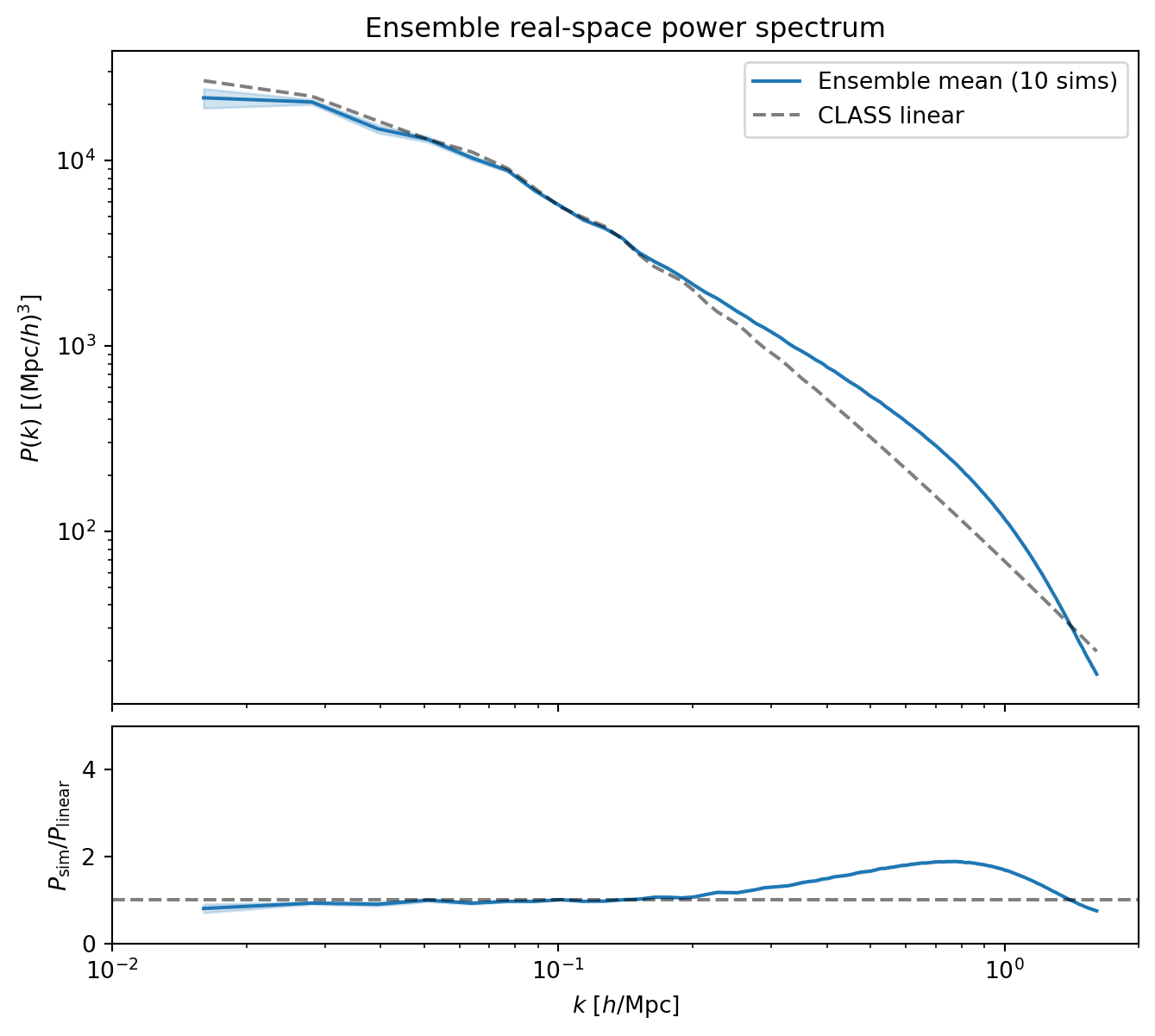
#| label: fig-ensemble-real-pk
#| fig-cap: "Ensemble mean of the real-space $P(k)$ compared to the CLASS
#| linear prediction. The error bars (standard error on the mean) are
#| much smaller than the single-realization scatter, confirming that the
#| ensemble average converges to the true power spectrum."
pk_class_ens = pk_of_k(np.array(k_ens))
pk_real_err = pk_real_std / np.sqrt(n_real)

fig, (ax1, ax2) = plt.subplots(2, 1, figsize=(8, 7),
                                gridspec_kw={'height_ratios': [3, 1], 'hspace': 0.05})

ax1.loglog(k_ens, pk_real_mean, 'C0-', lw=1.5, label=f'Ensemble mean ({n_real} sims)')
ax1.fill_between(k_ens, pk_real_mean - pk_real_err, pk_real_mean + pk_real_err,
                 color='C0', alpha=0.2)
ax1.loglog(k_ens, pk_class_ens, 'k--', lw=1.5, alpha=0.5, label='CLASS linear')
ax1.set_ylabel(r'$P(k)$ [(Mpc/$h$)$^3$]')
ax1.set_xlim(0.01, 2)
ax1.legend()
ax1.set_xticklabels([])
ax1.set_title('Ensemble real-space power spectrum')

ratio_ens = pk_real_mean / pk_class_ens
ax2.semilogx(k_ens, ratio_ens, 'C0-', lw=1.5)
ax2.fill_between(k_ens, (pk_real_mean - pk_real_err) / pk_class_ens,
                 (pk_real_mean + pk_real_err) / pk_class_ens, color='C0', alpha=0.2)
ax2.axhline(1.0, color='k', ls='--', alpha=0.5)
ax2.set_xlabel(r'$k$ [$h$/Mpc]')
ax2.set_ylabel(r'$P_\mathrm{sim} / P_\mathrm{linear}$')
ax2.set_xlim(0.01, 2)
ax2.set_ylim(0, 5)

plt.show()
```
At intermediate and high $k$, the ensemble mean shows the expected nonlinear
enhancement over CLASS. On large scales, where we expect agreement with
linear theory, the ensemble mean sits a few percent below CLASS. This is
a real effect: our finite time-stepping does not perfectly reproduce the
exact linear growth rate, leading to a small systematic deficit in the
evolved power. Production codes address this with more timesteps,
higher-order integrators, or more careful treatment of the drift and kick
factors.
The ensemble averaging also reveals the importance of large volumes.
With a single realization (Section 2), the sample variance at low $k$
was large enough to mask this systematic deficit — the noise was bigger
than the signal we are trying to see. Only by averaging over 10
realizations could we beat down the scatter enough to notice it. The
Quijote suite uses boxes 2× larger in each dimension
($L = 1\,h^{-1}$Gpc) and thousands of realizations, enabling
percent-level precision on clustering statistics.
#### Ensemble-Averaged 2D Correlation Function
Averaging the 2D correlation function $\xi(r_\perp, r_\parallel)$ across
realizations dramatically reduces noise, giving a much cleaner view of the
RSD anisotropy than the single-realization plot from Section 4.
```{python}
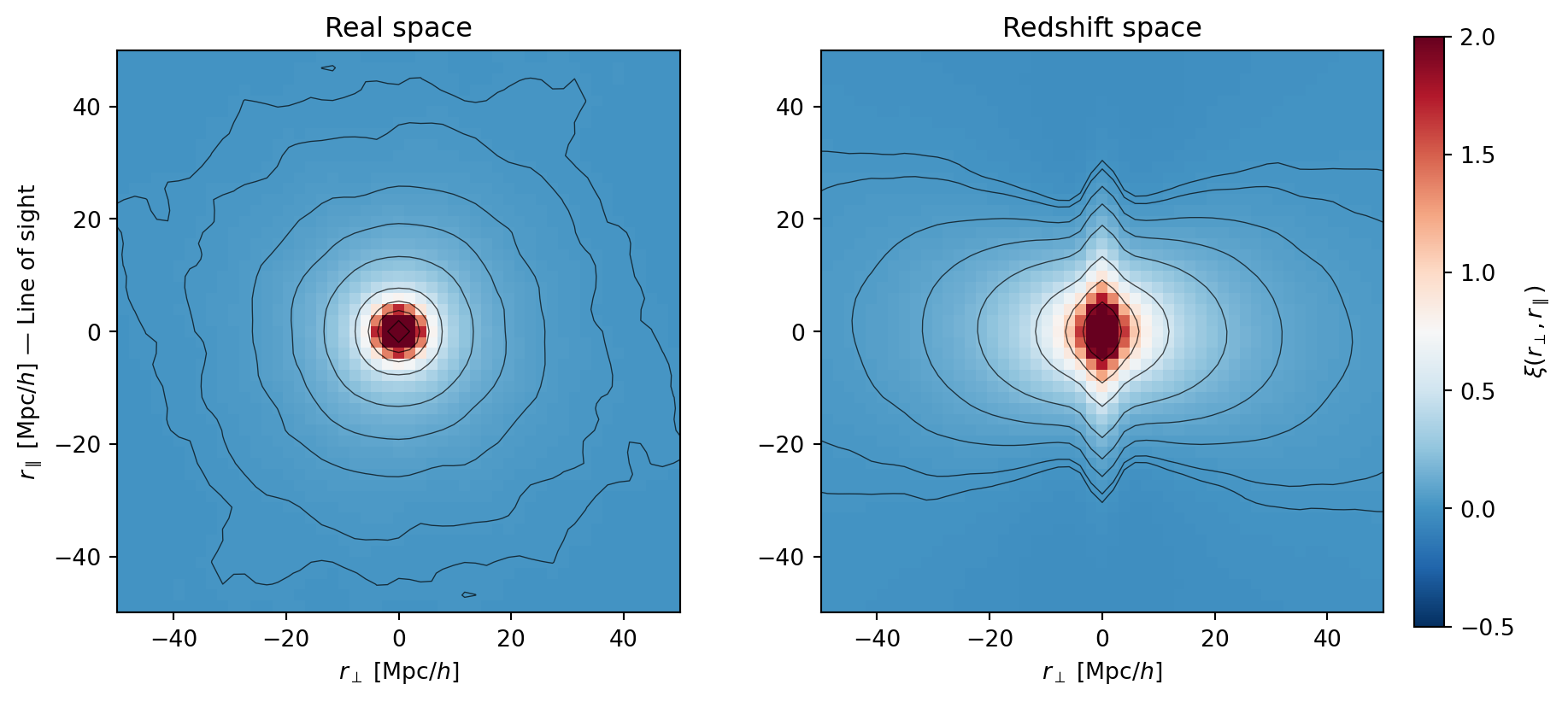
#| label: fig-ensemble-xi2d
#| fig-cap: "Ensemble-averaged 2D correlation function $\\xi(r_\\perp, r_\\parallel)$
#| in real space (left) and redshift space (right). Averaging over 10
#| realizations reveals clean, smooth contours. The Kaiser squashing
#| (compression along $r_\\parallel$) and Fingers of God (elongation at
#| small separations) are now clearly visible."
# Load xi_2d from ensemble
xi_real_stack = []
xi_rsd_stack = []
for i in range(n_real):
    d = np.load(os.path.join(ensemble_dir, f"real_{i:03d}.npz"))
    xi_real_stack.append(d['xi_real_2d'])
    xi_rsd_stack.append(d['xi_rsd_2d'])

xi_real_mean = np.mean(xi_real_stack, axis=0)
xi_rsd_mean = np.mean(xi_rsd_stack, axis=0)

# Coordinate arrays
r_vals = np.fft.fftshift(np.fft.fftfreq(Ng, d=1.0/L))
rmax = 50

levels = np.array([0.01, 0.02, 0.05, 0.1, 0.2, 0.5, 1.0, 2.0, 5.0])

fig, axes = plt.subplots(1, 2, figsize=(12, 5.5),
                         gridspec_kw={'wspace': 0.25})

for ax, xi, title in zip(axes, [xi_real_mean, xi_rsd_mean],
                          ['Real space', 'Redshift space']):
    im = ax.pcolormesh(r_vals, r_vals, xi.T, cmap='RdBu_r',
                       vmin=-0.5, vmax=2.0, shading='auto')
    ax.contour(r_vals, r_vals, xi.T, levels=levels,
               colors='k', linewidths=0.5, alpha=0.7)
    ax.set_xlim(-rmax, rmax)
    ax.set_ylim(-rmax, rmax)
    ax.set_xlabel(r'$r_\perp$ [Mpc/$h$]')
    ax.set_title(title)
    ax.set_aspect('equal')

axes[0].set_ylabel(r'$r_\parallel$ [Mpc/$h$] — Line of sight')
plt.colorbar(im, ax=axes, label=r'$\xi(r_\perp, r_\parallel)$',
             shrink=0.85, pad=0.02)
plt.show()
```
::: {.callout-note}
## Connection to Quijote
In Lectures 18–19, we analyzed power spectra from the Quijote simulation
suite — thousands of $N$-body realizations in $1\,(h^{-1}\text{Gpc})^3$
boxes with full $\Lambda$CDM gravity. What we have done here is the same
idea in miniature: multiple realizations of the same cosmology, used to
estimate the mean and variance of clustering statistics. The Quijote suite
uses larger boxes (better sampling of large-scale modes), higher resolution
(TreePM, not PM), and many more realizations — but the statistical
framework is identical.
:::