Code
import numpy as np
import matplotlib.pyplot as plt
from classy import Class
from scipy.integrate import quadThe correlation function \(\xi(r)\) is the 3D Fourier transform of the power spectrum \(P(k)\): \[ \xi(r) = \frac{1}{2\pi^2} \int_0^\infty k^2 P(k) \frac{\sin(kr)}{kr} dk \]
A word on the limits of integration here. While the limits formally run from \(0\) to \(\infty\), in practice, we often do not have the power spectrum defined at arbitrarily small or large \(k\). For a LCDM like power spectrum, the low-\(k\) limit is often not a concern, since the power is dropping off at large scales. The high-\(k\) limit is more tricky, since it is easy to get ringing artifacts in the correlation function if we truncate at too low a \(k\) value or too abruptly. In practice, we avoid this by smoothing the correlation function by truncating the integral with a Gaussian of scale \(R \sim 0.1-1 \, h^{-1} \, \text{Mpc}\). This does not affect the correlation function at large scales.
To compute the correlation function, we can use the scipy.integrate.quad function to perform the integral. Note that we need to do this for each value of \(r\) we want to compute \(\xi(r)\) at, which can be computationally expensive. (There are more efficient methods to do this [e.g. look up FFTLog]), but we’ll stick to the direct integration for simplicity.
We’ll also assume that we have a function P(k) that returns the power spectrum at a given \(k\).
Finally, we include a Gaussian smoothing factor in the integral to avoid ringing artifacts.
import numpy as np
import matplotlib.pyplot as plt
from classy import Class
from scipy.integrate import quad# correlation function - take in a P(k) function, a list of r values.
# add optional smoothing scale, a kmin and kmax for the integral limits.
def xi_of_r(r_values, pk_func, kmin=1e-4, kmax=1e2, smooth_R=0.5, epsabs=0.0, epsrel=1e-3, **kwargs):
"""
Compute the real-space correlation function xi(r) from a power spectrum P(k).
Parameters
----------
r_values : array-like
Radii r (in the same units as k^{-1}).
pk_func : callable
Function P(k) returning the power spectrum at wavenumber k.
kmin, kmax : float
Integration limits for k.
smooth_R : float
Gaussian smoothing scale R for exp[-(k R)^2] to suppress ringing.
epsabs, epsrel : float
Absolute and relative error tolerances for quad.
**kwargs : dict
Additional keyword arguments passed to scipy.integrate.quad, including:
- limit : int, maximum number of subdivisions (default 50 for quad, can increase here)
Returns
-------
xi : ndarray
Correlation function xi(r) for each r in r_values.
"""
r_values = np.atleast_1d(r_values)
# Set default limit if not provided
if 'limit' not in kwargs:
kwargs['limit'] = 100
def integrand(k, r):
kr = k * r
if kr < 1e-3:
# Use Taylor expansion for small kr to avoid numerical issues
sinc_kr = 1.0 - (kr**2) / 6.0 + (kr**4) / 120.0
else:
sinc_kr = np.sin(kr) / kr
window = np.exp(-(k * smooth_R)**2)
return k**2 * pk_func(k) * sinc_kr * window
xi_vals = np.zeros_like(r_values, dtype=float)
prefactor = 1.0 / (2.0 * np.pi**2)
for i, r in enumerate(r_values):
xi_vals[i] = prefactor * quad(integrand, kmin, kmax, args=(r,),
epsabs=epsabs, epsrel=epsrel, **kwargs)[0]
return xi_valsLet’s explore examples here.
We can now use our xi_of_r function to compute the correlation function for a LCDM power spectrum calculated using CLASS from the previous notebook.
We first compute a fiducial LCDM power spectrum at \(z=0\), and define a wrapper that returns \(P(k)\) in units of \((\mathrm{Mpc}/h)^3\) for \(k\) in \(h/\mathrm{Mpc}\).
# Create a CLASS instance and compute the matter power spectrum
cosmo = Class()
cosmo.set({
    'output': 'mPk',
    'h': 0.7,
    'omega_b': 0.02237,
    'omega_cdm': 0.1200,
    'A_s': 2.1e-9,
    'n_s': 1.0,
    'P_k_max_h/Mpc': 50.0,
    'z_max_pk': 0.0
})
cosmo.compute()

def pk_func_hmpc(k_h):
    """Return P(k) for k in h/Mpc, in units of (Mpc/h)^3."""
return cosmo.pk(k_h * cosmo.h, 0.0) * cosmo.h**3We evaluate \(\xi(r)\) from \(r=10\) to \(150\,\mathrm{Mpc}/h\) in \(\sim 2\,\mathrm{Mpc}/h\) bins.
r_values = np.arange(10.0, 150.0 + 1e-9, 2.0)
xi_values = xi_of_r(r_values, pk_func_hmpc, kmin=1e-4, kmax=5.0, smooth_R=1)We split the curve by sign so that the log scale remains well-defined.
pos = xi_values > 0
neg = xi_values < 0

plt.figure(figsize=(9, 6))
if np.any(pos):
    plt.loglog(r_values[pos], xi_values[pos], color='tab:blue', label=r'$\xi(r) > 0$')
if np.any(neg):
    plt.loglog(r_values[neg], -xi_values[neg], color='tab:orange', label=r'$|\xi(r)|$ (negative)')

plt.xlabel(r'$r$ [Mpc/h]', fontsize=13)
plt.ylabel(r'$|\xi(r)|$', fontsize=13)
plt.title(r'Correlation Function $\xi(r)$', fontsize=15)
plt.legend(fontsize=11)
plt.grid(True, alpha=0.3)
plt.tight_layout()
plt.show()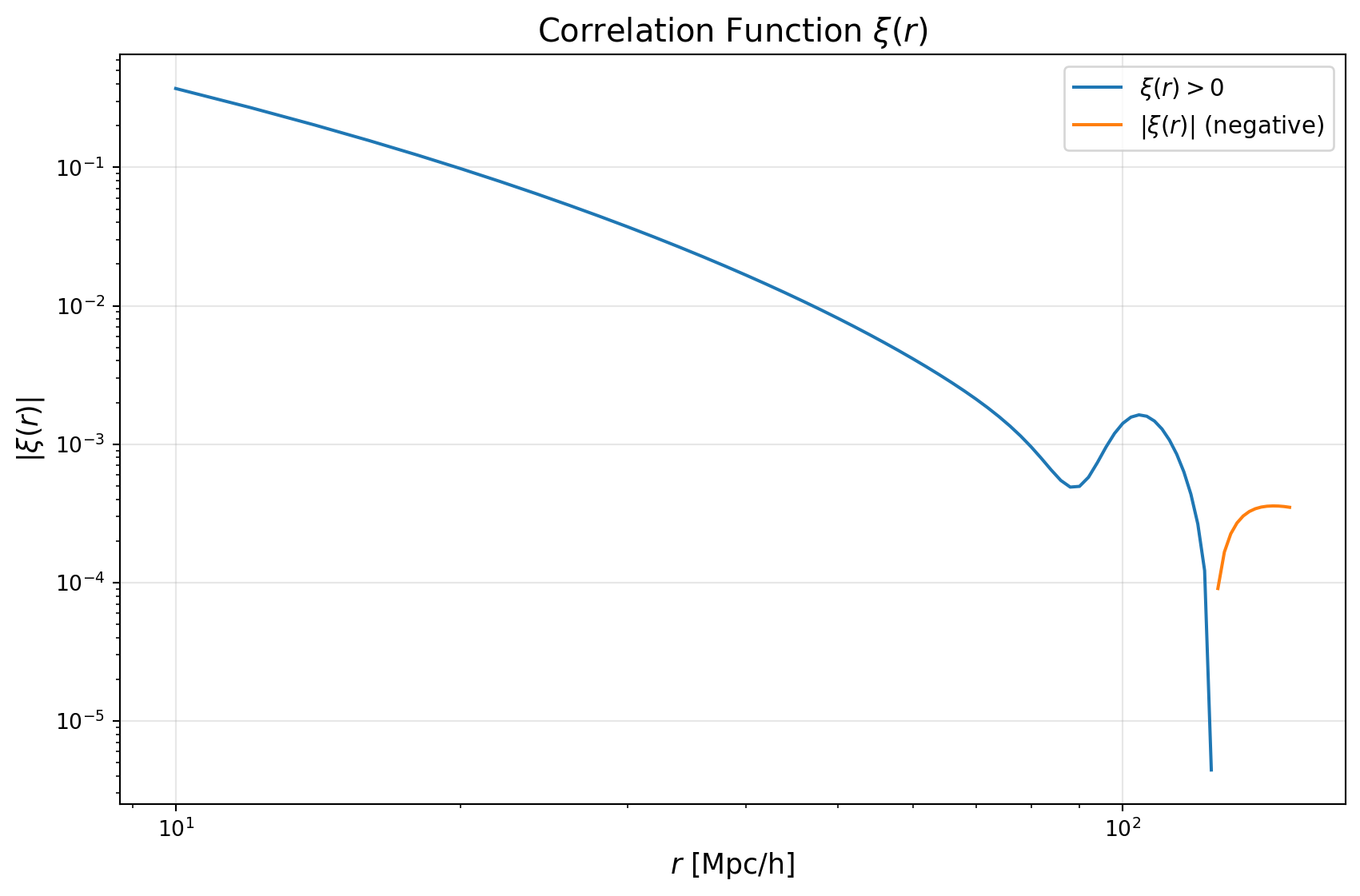
plt.figure(figsize=(9, 6))
plt.plot(r_values, r_values**2 * xi_values, color='black', linewidth=2)
plt.xlabel(r'$r$ [Mpc/h]', fontsize=13)
plt.ylabel(r'$r^2\,\xi(r)$', fontsize=13)
plt.title(r'$r^2\,\xi(r)$', fontsize=15)
plt.grid(True, alpha=0.3)
plt.tight_layout()
plt.show()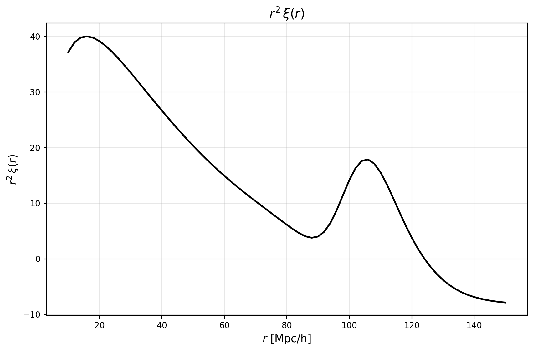
To see the effect of truncating the integral at too low a \(k\) value, we can compute \(\xi(r)\) with a much lower \(k_{\max}\) and compare to our previous result.
We compare three standard cases with different smoothing scales: \(R = 0.5\,\mathrm{Mpc}/h\), \(2.0\,\mathrm{Mpc}/h\), and \(4.0\,\mathrm{Mpc}/h\), all computed with the full \(k_{\max}=50\,h/\mathrm{Mpc}\).
We also show a pathological case where we truncate the integral at \(k_{\max}=1\,h/\mathrm{Mpc}\) with modest smoothing (\(R=0.5\,\mathrm{Mpc}/h\)). This demonstrates the characteristic oscillations that appear when the truncation is too aggressive—these are the ringing artifacts we discussed. In practice, this shows why careful choice of \(k_{\max}\) and smoothing scale is important when computing the correlation function from observationally-limited power spectrum measurements.
smooth_R_values = [0.5, 2.0, 4.0]
colors = ['tab:red', 'black', 'tab:blue']
labels = [rf'$R = {R}\,\mathrm{{Mpc}}/h$' for R in smooth_R_values]

plt.figure(figsize=(10, 6))

for smooth_R, color, label in zip(smooth_R_values, colors, labels):
    xi_smooth = xi_of_r(r_values, pk_func_hmpc, kmin=1e-4, kmax=50.0, smooth_R=smooth_R, limit=150)
    plt.plot(r_values, r_values**2 * xi_smooth, color=color, linewidth=2, label=label)

# Add truncated k_max case with ringing artifacts
xi_truncated = xi_of_r(r_values, pk_func_hmpc, kmin=1e-4, kmax=1.0, smooth_R=0.5, limit=150)
plt.plot(r_values, r_values**2 * xi_truncated, color='tab:orange', linewidth=2, linestyle='--',
         label=r'$k_{\max}=1\,h/\mathrm{Mpc}$, $R=0.5\,\mathrm{Mpc}/h$ (truncated)')

plt.xlabel(r'$r$ [Mpc/h]', fontsize=13)
plt.ylabel(r'$r^2\,\xi(r)$', fontsize=13)
plt.title(r'Effect of Gaussian Smoothing on $r^2\,\xi(r)$', fontsize=15)
plt.legend(fontsize=11)
plt.grid(True, alpha=0.3)
plt.tight_layout()
plt.show()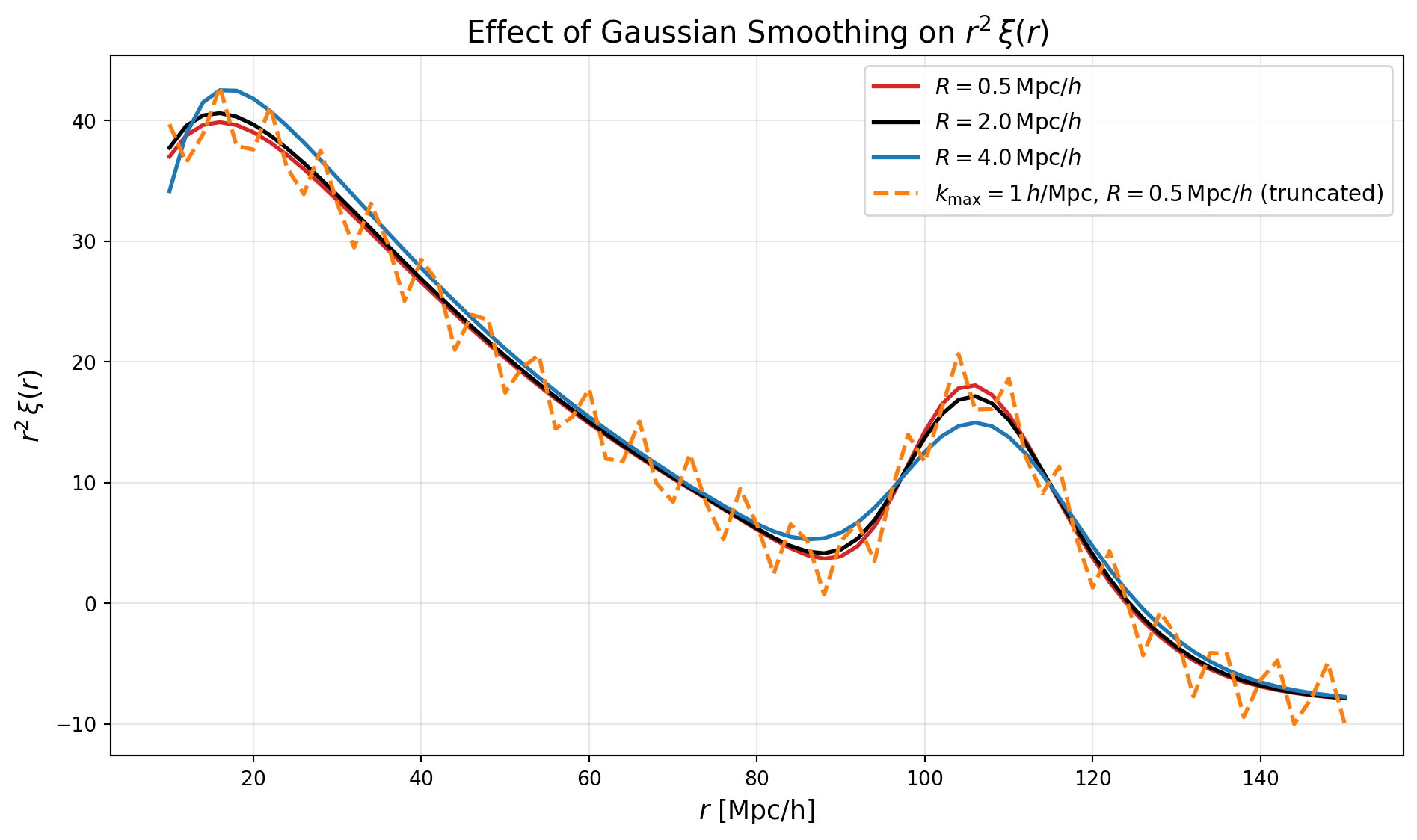
Let’s also compute the correlation function for a simple power-law spectrum \(P(k) = A\,k^{-n}\). This serves as a toy model that’s easier to understand analytically (though the real LCDM spectrum has more structure). We’ll compare this directly to the LCDM case.
Note that for the power-law case, the correlation function will also be a power-law in \(r\) \[ \xi(r) \propto r^{n-3} \]
# Define a power-law spectrum P(k) ~ k^{-1}
def pk_powerlaw(k):
    return 1.0 * k**(-1.0)

# Compute xi(r) for the power-law spectrum
xi_pl = xi_of_r(r_values, pk_powerlaw, kmin=1e-4, kmax=50.0, smooth_R=0.5, limit=150)

# Also compute LCDM with same smoothing for comparison
xi_lcdm = xi_of_r(r_values, pk_func_hmpc, kmin=1e-4, kmax=50.0, smooth_R=0.5, limit=150)

plt.figure(figsize=(10, 6))
plt.loglog(r_values, 400*np.abs(xi_pl), color='tab:green', linewidth=2, label=r'Power-law: $P(k) \propto k^{-1}$')
plt.loglog(r_values, np.abs(xi_lcdm), color='black', linewidth=2, label=r'LCDM')

plt.xlabel(r'$r$ [Mpc/h]', fontsize=13)
plt.ylabel(r'$|\xi(r)|$', fontsize=13)
plt.title(r'Comparison: Power-law vs LCDM Correlation Functions', fontsize=15)
plt.legend(fontsize=11)
plt.ylim(1e-4, 1)
plt.grid(True, alpha=0.3, which='both')
plt.tight_layout()
plt.show()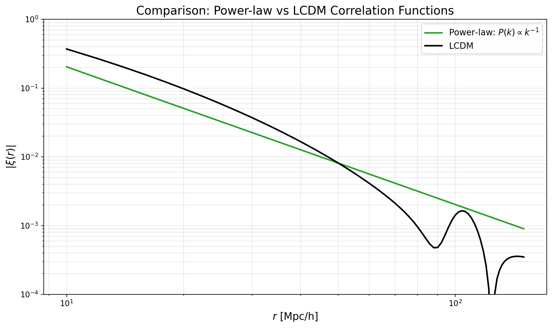
# Clean up CLASS
cosmo.struct_cleanup()